NONMEM Users Guide Part IV - NM-TRAN - Chapter III

III. Control Records

III.A. Record Syntax - General

A listing of NM-TRAN control record names and options is given in Appendix I. General rules for constructing these names and options are given in this section. The reader may refer to the example of the control records given in chapter I. It is not possible for NM-TRAN to generate a NONMEM control stream which contains syntax errors. Errors in an NM-TRAN control stream are reported in a report file; see Guide III.

E.g. $OMEGA

E.g. SIGDIGITS

 $COVAR

 $THETA  7   ;Mean Clearance

$THETA   7   ;Mean Clearance
        20   ;Mean Volume

E.g.
$THETA  7
        20

$THETA 7 20 .7
$OMEGA .5 4 .005

  MAXEVAL=400    SIGDIGITS=4, PRINT=5

and B is called the option value

  MAXEVAL = 400

 MAX = 300   or   MAX 300

In the descriptions of the particular records, which follow in later sections, square brackets are used to surround an option or group of options, none of which need actually appear in the record. If they surround a group of options, a vertical line is used to separate these options in the description, and at most one of the options may be selected to actually appear in the record. If none are selected to appear, then the default option

indicated in boldface (if there is an option so indicated), is understood to apply.

E.g. [UNCONDITIONAL|CONDITIONAL] indicates a choice between the options UNCONDITIONAL and CONDITIONAL, and if neither are selected to appear in the record, it is understood that the first option applies.

III.B. Record Syntax - Specific Records

Specific NM-TRAN control records are described in the next subsections.

III.B.1. $PROBLEM Record

$PROBLEM  text

E.g.
$PROB  THEOPHYLLINE   POPULATION DATA

The text becomes a heading for the NONMEM printout.

This record is required, and the first NM-TRAN control record must be a $PROBLEM record. A $PROBLEM record other than the first one marks the beginning of another problem specification.

The text must be contained on a single record, and only the first 72 characters of text (starting with the second character after the record name) are used in the heading. Spaces and semicolons in the text are included "as is".

III.B.2. $INPUT Record

$INPUT @item sub 1 ~ item sub 2 ~ item  sub 3 ~...@

E.g.
$INPUT      ID DOSE TIME CP=DV WT

The items define the data item types that appear in the NM-TRAN data records, as well as the order of their appearance.

This record is required, and it must precede any other NM-TRAN control record in the problem specification that refers to specific data item types.

Each item has form B or A=B, where A and B are data item labels. Each data item label consists of 1-4 letters (A-Z) and numerals (0-9), but it must begin with a letter. The labels may be used in subsequent NM-TRAN control records, and they will be used as labels for data items in NONMEM output.

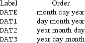
NM-TRAN recognizes certain reserved labels: ID, L1, L2, DV, MDV, TIME, DATE, DAT1, DAT2, DAT3, DROP.

If the user prefers to label a NONMEM data item type or a time data item type with a label (A) other than the reserved one (B), he may use the item A=B. In this case A is called a synonym for B. Alternatively, he may use the item B=A, i.e. the order of the labels A and B are reversed in the item so that the reserved label comes first. Either of the labels A and B may be used in subsequent control records of the problem specification. However, only the synonym is used as a label in NONMEM output. Both A and B can be reserved labels. Thus one type of data item can serve simultaneously as another type, e.g. ID=TIME. Another example of this is DATE=DROP.

The items DROP, A=DROP, or DROP=A are all equivalent. The label SKIP acts just as does the label DROP. The label DROP may not be used when the $DATA record contains a format specification (see section B.5).

Time data items are translated from clock times to relative times when at least one time data item contains a colon (:). Time data items are also translated from clock times to relative times when the reserved label DATE, DAT1, DAT2, or DAT3 is used. In this case the order of the fields (day, month, year) must be the same across all the date data items. This order corresponds to which label is used:

If only one field is used, it is assumed to be the day field. If two fields are used, they are assumed to be month and day fields. When two or more fields are used, the user should be careful to use, for example, DATE=DROP; otherwise, use of the nonumeric separator will raise an error during the NONMEM run.

If the data set is single-subject, ID data items are automatically generated, unless the reserved label L1 is used. A=L1 or L1=A can also be used. Generated ID data items are assigned the label .ID. (i.e. ID surrounded by dots). This label can be used in subsequent NM-TRAN control records of the problem specification.

Changes to the $INPUT record, may cause changes to generated codes. In this case care should be taken in using the previous load module.

INPT is an alias for INPUT.

III.B.3. $INDEX Record

$INDEX  [@label sub 1@|@value sub 1@]  [@label sub 2@|@value  sub 2@]  [@label sub 3@|@value sub 3@] ...

E.g.
$INDEX   DOSE  1

The labels are those of data items, as established by the $INPUT record. The values are integers no larger than the number of (non-DROP) items in the $INPUT record. Either (i) the index of the data items with label @label sub I@, or (ii) @value sub I@, whichever is chosen, is stored in INDXS(I). (The index of a data item is its position in the NONMEM data record.) For the above example, and using the $INPUT record shown in chapter I: INDXS(1)=2, and INDXS(2)=1.

This record is optional, and it need not appear unless some complete FORTRAN-coded subroutines are developed by the user, and at least one of these subroutines makes explicit use of the INDXS array.

INDXS is an array which is one of the arguments to certain user-supplied subroutines; see Guide I, section C.4.1, or Guide VI, sections III.C, IV.B, and VI.A. The array cannot be used with an abbreviated code. Therefore, the $INDEX record is not of interest to users of NM-TRAN who only use abbreviated codes.

In the above description INDXS(I) should be understood to always mean the Ith element of the INDXS array that is available to a user-written routine. With PREDPP the routine actually has access to only part of a larger INDXS array, only to elements 12-50 of the larger array. NM-TRAN stores the indices of certain data items of use to PREDPP in elements 1-11, but PREDPP renumbers elements 12-50 to 1-39 before passing INDXS as an argument to the routine.

$INDXS is an alias for $INDEX.

Commas between labels and values are optional.

III.B.4. $CONTR Record

$CONTR   DATA=([@label sub 1@|0] [@label sub 2@|0] [@label sub 3@|0])

E.g.
$CONTR    DATA=(0,TYPE)

This record defines one to three types of data items defined in the $INPUT record to be made available to subroutines CONTR, CCONTR, and MIX in the DATA array.

This record is optional and need only appear if the CONTR, CCONTR, or MIX subroutine is user-supplied and uses data items stored in the DATA array.

@label sub i@ is the label (or synonym) given in the $INPUT record for the ith data item type.

The CONTR and CCONTR subroutines are used to define an objective function which differs from the default (ELS) objective function. The MIX subroutine is used to describe the mixing parameter of a mixture model; see Guide VI, section III.L.2. More information about these routines may be obtained by consultation with the NONMEM Project Group. These routines are called with individual records. An array DATA is available in NONMEM read-only commons and changes value with each individual record. It contains up to three types of data items occuring in each observation record of an individual record. For any individual record, the data item occuring in the Ith observation record of the individual record, having the Jth label occuring in the DATA option of the $CONTR record, is available in DATA(I,J). If a 0 is used in the DATA option instead of a label, then a 0 is found in DATA(I,J).

Commas between labels and 0’s are optional.

III.B.5. $DATA Record

$DATA  [filename|*] [(format)] [IGNORE=@c sub 1@] [NULL=@c sub 2@] [NOWIDE|WIDE] [CHECKOUT]
       [RECORDS=@n sub 1@] [LRECL=@n sub 2@] [NOREWIND|REWIND]

E.g.
$DATA       DATAFILE

This record gives the name of the file containing the NM-TRAN data set.

This record is required with the first problem specification, and with any problem specification where the NM-TRAN data set differs from that of the preceding problem specification.

The filename must be the first option on the record. It may be enclosed by single quotes or by double quotes, in which case it can contain any special characters other than embedded spaces. If not enclosed by quotes, it must not contain embedded spaces, commas, semicolons, or parentheses.

If the $DATA record is missing from the problem specification, the problem uses the same NONMEM data set as that used in the previous problem. With the previous problem the user might have modified data items from those found in the NONMEM data set at the beginning of that problem (e.g. the modification may have occurred in the simulation step, or in the initialization/finalization step - see Guide II, section D.2.2, Guide VI, section VI.A), and then the data set used in the current problem (NONMEM’s internal copy of the data set) contains the modified data items. Using an asterisk in the $DATA record, in place of the file name, has the same effect as omitting the $DATA record. However, when one wants to use the CHECKOUT option, as well as use the NONMEM data set from the previous problem, the asterisk must be used. In this case no other options should be used.

The format refers to a FORTRAN format specification to be used by NM-TRAN to read the NM-TRAN data records. Note that this specification is to be enclosed in parentheses. Format codes F, E, and X may be used, but not I. The format will also be used by NONMEM to read the NONMEM data records, after it had been modified to account for generated data items. If a format is provided, the label DROP cannot be used, and the WIDE and NULL options may not be used. If a format is omitted, the NM-TRAN records can still be read, and a format specification which is appropriate for reading the NONMEM data records will be generated. In this case a NONMEM data set is found in FDATA (see section II.B).

When the character @c sub 1@ appears in column one of a (FORTRAN) record of the data set, this record does not appear in the NONMEM data set. Such records can serve as comment records in the NM-TRAN data set (see section II.C.3). The character @c sub 1@ can be any character other than a blank or semicolon. In the $DATA record it can be enclosed by single quotes or by double quotes, in which case a semi-colon is permitted.

Every occurrence in the NM-TRAN data set of a dot surrounded by blanks/commas, or of consecutive commas, is replaced by a null data item in the NONMEM data set. Null data items are also supplied for data items that are missing from the end of an NM-TRAN data record (there may be several missing from the end of any given record) but that are defined in the $INPUT record. This null data item consists of the specified character @c sub 2@, and it occupies the last position in the field of the NONMEM data set into which it is placed. The character @c sub 2@ can be enclosed by single quotes or by double quotes. The default for @c sub 2@ is a blank.

The option NOWIDE specifies that the FORTRAN records of the NONMEM data set, generated by NM-TRAN, are to consist of 80 characters. In order to accomplish this NM-TRAN may need to suppress space between fields or generate multi-line NONMEM data records. The option WIDE specifies that only single-line NONMEM data records are to be generated. These records always include at least one space between fields. With this option the NONMEM data records can be no longer than 300 characters, and they can number no more than 9999. They comprise a NONMEM data set which may be more legible than one obtained without using WIDE, and which can be processed by a program other than NONMEM.

The option CHECKOUT specifies that NONMEM is to run in data checkout mode. In this mode, tables and scatterplots can be requested, so that the data (as "understood by NONMEM") can be examined, but no computations involving the model are performed, so that this examination cannot be hindered by problems with the logic in user-written routines or abbreviated codes. These routines and codes need only be syntactically correct. The predictions, residuals, weighted residuals, ETA’s and PRED-defined items that are displayed in tables and scatterplots (see sections B.16 and IV.F) are all 0. CHECKDATA can be used as an alias.

When the RECORDS option is used, the number @n sub 1@ is the number of data records in the NM-TRAN data set. This number must be less than 10,000. When the option is omitted, then there is no limit to the number of data records in the NM-TRAN data set. In this case the file is read to a FINISH record (see below), or to the physical end of file, whichever comes first. However, if there are 10,000 or more records, then it is suggested that a FINISH record be used since in this case and when, moreover, the NONMEM data set happens to coincide with the NM-TRAN data set, the NONMEM data set needs a FINISH record.

The length of a data record in the NM-TRAN data set cannot exceed 300 characters.

The LRECL option is only needed when the format is omitted, and when either (i) the operating system (e.g. IBM/CMS) raises a fatal error when a FORTRAN program tries to read more characters from a logical record than the number of characters in the record, or (ii) the operating system imposes a maximum record length which is smaller than 300 characters (e.g. CRAY/CTSS). The number @n sub 2@ is the number of characters in the NM-TRAN data records.

NOREWIND specifies that the file is not to be rewound before it is read, and REWIND specifies that the file is to be rewound. These options are ignored if used on the $DATA record appearing in the first problem specification of the NM-TRAN control stream, or on a $DATA record appearing in a subsequent problem specification when this record contains a file name different from that contained on the $DATA record of the prior problem specification. In these cases the file is automatically rewound. The REWIND and NOREWIND options are significant only when there are multiple problem specifications in the NM-TRAN control stream, and when the $DATA records appearing in two consecutive problem specifications, corresponding to two problems A and B, contain the same file name. In this situation:

Translation of NM-TRAN data records is a slower process than is translation of NM-TRAN control records. However, usually during a data analysis, changes are made to the NM-TRAN control records between runs, but not to the NM-TRAN data records. With large data sets once translation of the data records has been performed successfully, the output in FDATA can be stored (in a file of a different name) and used with subsequent NM-TRAN runs. In a subsequent run, use the format specification and value for @n sub 1@ found in the problem summary pages of the NONMEM output from the first run. If data items were dropped or generated, then use the list of "LABELS FOR DATA ITEMS", found in this earlier output, for the list of labels needed in the $INPUT record. If the data set is single-subject, and ID data items were generated, use L1 for the label of these data items.

$INFILE is an alias for $DATA.

When a format is omitted, a FINISH record consists of the characters FIN appearing anywhere in the record (the other characters are all blank). When a format is provided, a FINISH record must have the form described in Guide II, section D.2.3.

III.B.6. $SUBROUTINES Record

$SUBROUTINES  [@subname sub 1 = name sub 1@] [@subname sub 2 = name sub 2@] ...
              [SUBROUTINES=kind]

E.g.
$SUBROUTINES    PRED=pred

This record gives names associated with any subroutines which are user-supplied, i.e. for which abbreviated codes are not given. At the time NM-TRAN is installed the user chooses whether user-supplied FORTRAN codes are to be included in the FSUBS file. Inclusion is the installation default option (see Guide III). If this option is chosen, the names given in the $SUBROUTINES record are needed for the purpose of implementing this option. Otherwise, these names are only needed so that they can be listed in the FREPORT file. This file is needed only for documentation purposes, although it also can be used as input to a program that creates system commands for running NONMEM. The $SUBROUTINES record also indicates whether abbreviated codes which appear in the control stream are used to generate subroutines or whether they are used to generate Library instructions for NM-TRAN Library subroutines.

This record is only required with the first problem specification, and then only if the record contains some option. It applies to all problem specifications in the control stream, and it must not appear with a problem specification other than the first.

A subname may be chosen from the list: PRED, CRIT, CONTR, CCONTR, MIX, CONPAR. These subnames stand for NONMEM subroutines, any one of which can be user-supplied. The name to which it is set equal can be any 1-8 alphanumeric character string (periods and colons are also allowed) which begins with a letter. This is the name used in FREPORT. The name could be the same as the subname, but a subname is generic, and a name which is more specifically related to the actual code comprising the subroutine can be more useful. If user-supplied source codes are included in FSUBS, then the names should be names of the files containing these codes. One subname-name pair should be used for each subroutine which is user-supplied.

There may exist one or more "other" user-supplied subroutines used by one of the subroutines listed above. The special subname OTHER can be used in conjunction with such a routine; it is set to a name for the routine. (Such a subroutine B, called by subroutine A, can be included in the file containing A. In this case OTHER would not be set to a name for B.) Unlike the other subnames, OTHER can appear up to three times in the $SUBROUTINES record, and used for up to three different user-supplied routines.

If the PRED subroutine is not user-supplied, so that PRED is not used as a subname, then an abbreviated code must be given for PRED (unless PREDPP is used; see chapter V).

Abbreviated codes cannot be given for the CRIT, CONTR, CCONTR, MIX, or CONPAR routines. If one of these routines is used, it must be supplied by the user.

SUBS is an alias for SUBROUTINES, L is an alias for LIBRARY, SP and S are aliases for SINGLE, and DP and D are aliases for DOUBLE.

The SUBROUTINES option may be coded with the part SUBROUTINES= missing.

E.g.
$SUB  SP

III.B.7. $ABBREVIATED Record

$ABBREVIATED  [COMRES=@n sub 1@] [COMSAV=@n sub 2@] [DERIV2=NO] [DERIV2=NOCOMMON]

E.g.
$ABBREVIATED    COMRES=2

This record gives attibutes which apply to all abbreviated codes.

This record is optional and may only appear if abbreviated codes appear. Then it only should appear with the first problem specification, and before any abbreviated code.

One use of the option COMRES involves the presence of both abbreviated and user-supplied subroutines. Values for variables defined in abbreviated codes may be displayed in tables and scatterplots. These variables are listed (i.e. their values are stored) in a NONMEM (named FORTRAN) common NMPRD4 in the generated or Library subroutine. User-supplied FORTRAN routines may also list variables whose values are to be displayed in this common. The first @n sub 1@ positions in the common are reserved for the use of these routines; generated and Library subroutines will not list variables defined in abbreviated codes in these positions. If there are no abbreviated codes, not only is COMRES not needed for this purpose, it may not be used. All variables listed in the common must be double precision variables if double precision NONMEM is used; otherwise, they must be single precision variables. The number @n sub 1@ can be nonnegative, and if the option is not used, it is understood to be 0. It can also be -1, in which case no variables defined in abbreviated codes are listed in the common. In this regard, see also section IV.H.

All variables defined in an abbreviated code are listed in NMPRD4, whether or not their values are displayed. Thus with PREDPP, where there may be more than one abbreviated code, each such variable is recognized as the same variable in all abbreviated codes in which it is used. If it desireable to avoid this type of global definition, then the option value -1 can be used. See also section IV.H.

The option COMSAV may be used when the variable COMACT is used in abbreviated code (see section IV.E.2). In this case the option COMRES should also be used, and @n sub 2@ must satisfy @0~<=~n sub 2~<=~n sub 1@.

The next two options primarily concern ways to avoid changing and recompiling NM-TRAN or NONMEM source code when NM-TRAN produces error messages indicating that certain internal table sizes are found to be too small for a given problem; see Guide III. In this regard, the option COMRES=-1 can also be useful (see also section IV.H).

When the option DERIV2=NO is used, code or Library instructions to compute second-partial derivatives with respect to @eta@ variables is not generated from abbreviated codes. These derivatives are only needed when the Laplacian estimation method is used (see section B.14). So in order to save CPU time one might be tempted to use this option when the Laplacian method is not used. However, when the Laplacian method is not used, the code computing the second derivatives is never executed. Therefore usually, there is little reason to include the option. It is generally recommended that the option not appear, so that with generated subroutines, a load module that computes these derivatives can also be used in a subsequent run which uses the Laplacian method. If it does appear, if PREDPP is not used, and if the Laplacian estimation method is requested in a subsequent run using the same load module, then, in effect, the first-order conditional estimation method is used in that run, although using somewhat more computer time than is necessary. However, care should be taken to avoid this situation. If the option appears, and PREDPP is used, then the Laplacian estimation method must not be requested in a subsequent run using the same load module, even when all second-partial derivatives that might be computed are uniformly zero (in which case code computing these zeros is actually not generated whether or not the option appears).

Values of second-partial derivatives of a variable defined in an abbreviated code are stored in other variables defined in the generated or Library routine. Normally, these variables are listed are also listed in common NMPRD4 (see above). When the option DERIV2=NOCOMMON is used, these variables are not listed in the common. In this case these variables are not displayable. In this case also, if PREDPP is used, no variable defined in the abbreviated code for PK, may be referenced in the abbreviated code for ERROR.

III.B.8. $PRED Record

$PRED
         the abbreviated code

This record gives an abbreviated code for the PRED routine. The syntax of an abbreviated code is described in chapter IV.

This record is optional. If it appears, it must be with the first problem specification, and only with this problem specification.

III.B.9. $THETA Record

$THETA  @value sub 1@  [@value sub 2@]  [@value sub 3@] ...
        [NUMBERPOINTS=n] [ABORT|NOABORT]

E.g.
$THETA  (.1,3.,5.)  (.008,.08,.5) (.004,.04,.9)

This record gives initial estimates for @theta@’s, as well as bounds on the final estimates.

This record is required only if the statistical model contains @theta@ parameters (most models do). When a $MSFI record appears in the problem specification, the $THETA record should not appear.

A value has one of three forms:

where init is the initial estimate, and low and up are lower and upper bounds respectively. The lower bound can be -INF, i.e. @- inf@, and the upper bound can be INF, i.e. @inf@, unless form 3 is used, in which case both bounds must be finite numbers. Form 3 is used when the user requires some help in obtaining an initial estimate for the parameter. Usually, though, the user should be able to develop a reasonable initial estimate, and when he can, there is some savings in computation time. An initial estimate equal to 0 is not allowed, unless the FIXED option is used. Use of this option indicates that the final parameter estimate is to be constrained to equal the initial parameter estimate. If this option is used with form 2, then low, init and up must all be equal. There may be at most 20 values.

Another example:

$THETA  3 FIXED  (-INF,.08,.5) (.004,,.9)

where the three forms used are 1,2 and 3, in that order.

Parentheses around init with form 1 are optional. The designation INF can also be coded INFINITY, INFIN, or 1000000. The character +’ can precede INF, as can the character ’-’. Integers need not have decimal points.

If form 3 is used, a search for an initial estimate is undertaken by NONMEM (not NM-TRAN). A number of points in a subspace of the @theta@ parameter space will be examined. This subspace consists of the multidimensional rectangle formed by the lower and upper bounds for all parameters whose values are of form 3. The number of points examined will be automatically determined by NONMEM, or it can be specified by the number n with the NUMBERPOINTS option. The options ABORT and NOABORT apply during the search. For information concerning these option, see section IV.G.

Aliases for NUMBERPOINTS are: NUM, NUMPTS, NUMBERPTS. This option can occur at the end of the record, or at the beginning, or between two values. THTA is an alias for THETA.

Commas between values are optional, except with form 3.

III.B.10. $OMEGA Record

$OMEGA  [DIAGONAL(n)|BLOCK(n)|BLOCK(n) SAME|BLOCK SAME]
        [[@value sub 1@]  [@value sub 2@]  [@value sub 3@] ... [FIXED]]

E.g.
$OMEGA BLOCK(3)  6. .005 .3 .0002 .006 .4

This record gives initial estimates for elements of the @OMEGA@ matrix, i.e. the variances and covariances of the @eta@ variables in the statistical model. Constraints on @OMEGA@ are also indicated.

This record should appear only if the statistical model contains @eta@ variables. If it appears, then there must be one such record corresponding to each block of @OMEGA@, and the order of these records in the control stream must correspond to the order of the blocks. The values in an $OMEGA record are the initial estimates for the elements of the corresponding block. Under some circumstances $OMEGA records may or may not appear, and the equivalent effect is achieved in either case (see below). When a $MSFI record appears, no $OMEGA records should appear. When PREDPP is used, and a $PK record does not appear, while a $ERROR record does appear, certain care must be taken with the $OMEGA record; see section V.6.

@OMEGA@ can be considered to be in block diagonal form with blocks @B sub 1@, @B sub 2@, ..., @B sub m@ (submatrices of @OMEGA@):

This form need not be unique, and there may be only one block (which is most usual). The following description applies to the @i@th block, @i~=~1, ... , m@.

If the DIAGONAL option is used, it must precede the values. In this case @B sub i@ is constrained to be diagonal, and the values are the initial estimates of its diagonal elements given in the diagonal order. The number n is the dimension of @B sub i@; it must not exceed 10. In addition, a final estimate of an individual element of a diagonal block can be constrained to be equal to the initial estimate of the element by using the FIXED option. The value giving the initial estimate should be coded with any one of the forms:
init FIXED
(init FIXED)
(FIXED init)

If the BLOCK option is used, it must precede the values. In this case the form of @B sub i@ is unconstrained, and the values are the initial estimates of its lower triangle elements given in row-wise order. The number n is the dimension of @B sub i@; it must not exceed 5. If FIXED option is used, all the final estimates of the elements of @B sub i@ are constrained to be equal to the initial estimates of these elements.

If the BLOCK(n) SAME or BLOCK SAME option is used, @B sub i@ is constrained to be equal to @B sub i-1@. In this case @i@ must be greater than 1, the number n (if it is given) must be the dimension of @B sub i-1@, and values are not given.

If some of the values in a record are omitted (other than a record with the BLOCK(n) SAME or BLOCK SAME option), then all values in the record must be omitted, and NONMEM will try to obtain initial estimates for the elements of the block. In this case, if the DIAGONAL option is used, it must appear explicitly in the record. Often, though, the user should be able to develop reasonable initial estimates, and when he can, there may be a little savings in computation time.

If no $OMEGA records appear, if no $MSFI record appears, but @eta@ variables are used in an abbreviated code, then it is assumed that a record

$OMEGA  DIAGONAL(n)

where n is the largest index used with an @eta@ variable in all abbreviated codes, might have equivalently been used. (If, though, with PREDPP an abbreviated code for PK is not used, while an abbreviated code for ERROR is used, see section V.6.)

With the BLOCK option, the FIXED option can occur anywhere among the list of values. These values (of the lower triangle) are given in row-wise order, i.e. @B sub {i,11}@, @B sub {i,21}@, @B sub {i,22}@, ..., @B sub {i,n1}@, @B sub {i,n2}@, ..., @B sub {i,nn}@.

Commas between values are optional.

An initial estimate of an element of a diagonal block must be >0, or it can be 0 if the FIXED option is used with it. An initial estimate of a non-diagonally-constrained block must be positive definite, or it can be (uniformly) 0 if the FIXED option is used with it. (In any case the initial estimates of @OMEGA@ and @SIGMA@ cannot both be 0 unless the Simulation Step is the only step implemented.)

The NM-TRAN translation of $OMEGA records is such that new blocks in addition to @B sub 1@, @B sub 2@, etc. may be created. This should be transparent to the user, except that he will see additional blocks listed in the problem summary output by NONMEM.

III.B.11. $SIGMA Record

$SIGMA  [DIAGONAL(n)|BLOCK(n)|BLOCK(n) SAME|BLOCK SAME]
        [[@value sub 1@]  [@value sub 2@]  [@value sub 3@] ... [FIXED]]

E.g.
$SIGMA  .4

This record gives initial estimates for elements of the @SIGMA@ matrix, i.e. the variances and covariances of the @epsilon@ variables in the statistical model. Constraints on @SIGMA@ are also indicated.

This record should appear only if the statistical model contains @epsilon@ variables. If it appears, then there must be one such record corresponding to each block of @SIGMA@, and the order of these records in the control stream must correspond to the order of the blocks. The values in an $SIGMA record are the initial estimates for the elements of the corresponding block. Under some circumstances no $SIGMA records need appear (see below). When a $MSFI record appears, no $SIGMA records should appear.

@SIGMA@ can be considered to be in block diagonal form with blocks @B sub 1@, @B sub 2@, ..., @B sub m@ (submatrices of @OMEGA@):

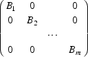
This form need not be unique, and there may be only one block (which is most usual). The following description applies to the @i@th block, @i~=~1, ... ,m@.

If the DIAGONAL option is used, it must precede the values. In this case @B sub i@ is constrained to be diagonal, and the values are the initial estimates of its diagonal elements given in the diagonal order. The number n is the dimension of @B sub i@; it must not exceed 10. In addition, a final estimate of an individual element of a diagonal block can be constrained to be equal to the initial estimate of the element by using the FIXED option. The value giving the initial estimate should be coded with any one of the forms:
init FIXED
(init FIXED)
(FIXED init)

If the BLOCK option is used, it must precede the values. In this case @B sub i@ is unconstrained, and the values are the initial estimates of its lower triangle elements given in row-wise order. The number n is the dimension of @B sub i@; it must not exceed 5. If FIXED option is used, all the final estimates of the elements of @B sub i@ are constrained to be equal to the initial estimates of these elements.

If the BLOCK(n) SAME or BLOCK SAME option is used, @B sub i@ is constrained to be equal to @B sub i-1@. In this case @i@ must be greater than 1, the number n (if it is given) must be the dimension of @B sub i-1@, and values are not given.

If some of the values in a record are omitted (other than a record with the BLOCK(n) SAME or BLOCK SAME option), then all values in the record must be omitted, and NONMEM will try to obtain initial estimates for the elements of the block. In this case, if the DIAGONAL option is used, it must appear explicitly in the record. Often, though, the user should be able to develop reasonable initial estimates, and when he can, there may be a little savings in computation time.

If no $SIGMA record appears, if no $MSFI record appears, but @epsilon@ variables are used in an abbreviated code, then it is assumed that a record

$SIGMA  DIAGONAL(n)

where n is the largest index used with an @epsilon@ variable in the abbreviated code, might have equivalently been used.

With the BLOCK option, the FIXED option can occur anywhere among the list of values. These values (of the lower triangle) are given in row-wise order, i.e. @B sub {i,11}@, @B sub {i,21}@, @B sub {i,22}@, ..., @B sub {i,n1}@, @B sub {i,n2}@, ..., @B sub {i,nn}@.

Commas between values are optional.

An initial estimate of an element of a diagonal block must be >0, or it can be 0 if the FIXED option is used with it. An initial estimate of a non-diagonally-constrained block must be positive definite, or it can be (uniformly) 0 if the FIXED option is used with it. (In any case the initial estimates of @OMEGA@ and @SIGMA@ cannot both be 0.)

The NM-TRAN translation of $SIGMA records is such that new blocks in addition to @B sub 1@, @B sub 2@, etc. may be created. This should be transparent to the user, except that he will see additional blocks listed in the problem summary output by NONMEM.

III.B.12. $MSFI Record

$MSFI   filename [NORESCALE|RESCALE] [NPOPETAS=n]

E.g.
$MSFI   MSF13

This record gives the name of a Model Specification File to be input. Such a Model Specification File is a file output by a previous NONMEM run, which contains certain model information pertaining to that run. It also contains other information which allows (i) the minimization search in that run, if terminated unsuccessfully because the limit on the allowable number of objective function evaluations was attained, to be smoothly continued in the current run, and (ii) Covariance, Table, and Scatterplot Steps in the current run, which follow the successful termination of that search (in the current run or the previous run) to be implemented.

This record is required only if a Model Specification File is to be input. With PREDPP, if a $PK record is not used, while a $ERROR record is used, the $MSFI record must precede the $ERROR record.

The filename must be the first option on the record and must not contain embedded spaces, commas, semicolons, or parentheses.

If the search is continued in the current run (see section B.14), use of the NORESCALE option means that the search is continued just as it would have been continued in the previous run had the limit on the number of function evaluations not been attained. Use of the RESCALE option means that before the search is continued, the final estimates of the STP (see Guide I, section C.3.5.1) from the previous run are rescaled so that they are all 0.1 (see Guide II, section F).

When the $MSFI record is used in a problem specification, $THETA, $OMEGA, and $SIGMA records should not appear for that specification.

The number n with the NPOPETAS option is the number of @eta@ variables used with population data. When n is 0, then the data are regarded as single-subject data (see section II.C.4). It is a good practice to include the NPOPETAS option; it is a simple thing to do. However, the NPOPETAS option is only needed when the data should be regarded as population data and: (i) a $PRED record is not used and the label L1 is not used in the $INPUT record (or if PREDPP is used, (ii) $PK and $ERROR records are not used and the label L1 is not used in the $INPUT record, or (iii) a $PK record is not used, while a $ERROR record is used).

POPETAS or any of its abbreviations are aliases for NPOPETAS.

III.B.13. $SIMULATION Record

$SIMULATION  (seed1 [seed2] [NORMAL|UNIFORM] [NEW]) ...
             [SUBPROBLEMS=n] [ONLYSIMULATION] [OMITTED]

E.g.
$SIMULATION     (889215690) (2239177789 UNIFORM)

This record requests that the Simulation Step be implemented.

This record is optional.

Data are generated according to a statistical model. The DV data items of (NONMEM’s internal copy of) the data set are replaced by generated DV items. The model is that specified in the code for PRED (for PK, ERROR, etc. if PREDPP is used). The data are simulated using the parameter values given as initial estimates; see sections B.9-11. Initial estimates must be given for all parameters of the model.

The model used for data simulation may be complicated. It may involve covariables and random interindividual and intraindividual random effects. It may be the very model used for data analysis. One reason to simulate with such a model is to explore the information content of data obtained according to some particular design. The design is encoded into the data set. The Simulation and Estimation Steps, and possibly the Covariance Step too, are implemented, so that one can assess how well the true parameter values of the data analysis model can be estimated. This technique can be used during the course of a data analysis when the adequacy of the design has become suspect. However, it can also be used before the data are actually obtained to explore design choices.

If only a simulation of the structural part of the model is desired, i.e. the model without statistical components, the model need not involve random effects. In this case the $SIMULATION record need not even appear. If it does appear, the DV items are replaced with generated DV items based only on the structural model. If it does not appear, the DV items are not replaced, but prediction items, i.e. predictions returned by PRED, may still be displayed. To simulate only the structural part of the model when a full statistical model has already been specified, fix the initial estimates of the variances of the random effects, i.e. the initial estimates of @OMEGA@ and @SIGMA@, to zero.

Data can be simulated with one model and analyzed with another. There are two approaches. With the first approach, data are simulated in the Simulation Step and output in the Table Step (see section B.16). The table serves as the data set for a subsequent NONMEM run. (The DROP label can be used with the prediction, residual, and weighted residual data items of the table; see section B.2.) In the subsequent run the data are analyzed using the analysis model. With the second approach, codes for both models are given in PRED, but with any particular call to PRED, one or the other code is executed according to the value of a special variable (ICALL) that signals whether PRED is being called during the Simulation Step or a data analysis step (see section IV.D). The advantage of the first approach is that it is a bit more flexible. The advantage of the second is that data sets and the analyses performed on them can be more easily replicated; see the discussion below concerning the option SUBPROBLEMS.

A random source is an infinite sequence of pseudo-random numbers. At most 10 random sources can be defined for a single problem. The sources are numbered according to the ordering of their definitions in the record. The information coded within each set of parentheses defines the attributes of a single random source. A random source can be used with the problem for which it is defined. The same source can be defined for different problems. A source defined for one problem can be continued in a subsequent problem; see below. Unless a random source is explicitly defined for a given problem, it cannot be used with that problem.

When the model, i.e. either the simulation model or the data analytic model, uses @eta@ variables, or both @eta@ and @epsilon@ variables, and the Simulation Step is implemented, at least one random source must be defined (unless the variances of these variables are 0; see below). When the model is a mixture model and the Simulation Step is implemented, at least one random source must be defined. The first source is used by NONMEM to generate realizations of the @eta@ and @epsilon@ variables and/or to randomly mix individuals into different subpopulations according to the mixing parameter. Only the NORMAL attribute can be used with this source, i.e. during simulation the @eta@ and @epsilon@ variables are understood to be normally-distributed. (Mixing, though, does not involve normal pseudo-random numbers.) The NEW attribute cannot be used with any source other than this first source (see below).

The remaining defined random sources are used exclusively by the PRED subroutine (by the PK and ERROR subroutines if PREDPP is used). If no @eta@ variables appear in the model and a mixture model is not used, then all defined random sources can be used by PRED. On the other hand, in this case, no sources need even be defined. If @eta@ (and possibly @epsilon@) variables appear in the simulation model, but the initial estimates of @OMEGA@ (and @SIGMA@) are 0, and if a mixture model is not used, then again, no sources need be defined. A random source not used by NONMEM per se is called a user random source Such a source can use either the NORMAL or UNIFORM attribute (see below).

Numbers from user random sources are obtained via the NONMEM utility RANDOM. An abbreviated code can use RANDOM only when verbatim code is included (see section IV.I). A user-supplied FORTRAN code can use RANDOM by executing the FORTRAN statement

CALL RANDOM (K,R)

Each time RANDOM is called with K set to the index of a given user source, the routine returns the next number from that source. This number is returned in R, and is always a single-precision number.

Seed1 and seed2 together initiate the random source. Seed2 is used only seldomly (see below), and each seed is an integer between 0 and 21474836447. Two sources are the same if they are initiated with the same seeds.

Suppose that the current problem specification is not the first problem specification in the control stream, that the source is the ith source, @S sub i@, and that the last problem to use as many as i sources was problem number m. Then seed1 can be -1, indicating that @S sub i@ is the continuation of the ith source, @R sub i@, defined with problem m. That is, if the last number used from @R sub i@ was @x sub k@, then @S sub i@ is the infinite tail sequence of @R sub i@ starting with @x sub k+1@.

Seed2 is used when it is desired that the current problem make use of a continuation of a random source defined in a preceding NONMEM run. Examine the NONMEM output from the Simulation Step of the last problem in the earlier run using this source. Two ending seeds are printed in this output; often the second seed is 0. The continuation in the current problem is defined using these two seeds as seed1 and seed2. When the second seed is 0, it need not be given.

Use of the NORMAL option means that the numbers of the source are to be pseudo-normal with mean 0 and variance 1 (unless the source is the first and used to generate @eta@ and @epsilon@ realizations, in which case the variance-covariance of these variables is that specified in the $OMEGA and $SIGMA records). Use of the UNIFORM option means that the numbers of the source are to be pseudo-uniform on the interval [0,1].

During the Simulation Step PRED has access to simulated values for the @eta@ variables via the NONMEM utility routine SIMETA. When PRED is called with a data record from a given individual record, PRED can execute the FORTRAN statement

CALL SIMETA (ETA)

which results in appropriate values being stored in the one-dimensional ETA array; see section IV.A. These values will arise from a multivariate normal pseudo-random distribution with mean 0 and variance-covariance as specified with the $OMEGA record. By default, no matter how many times this statement is executed, as long as the individual record is the same, the same values are stored. If, though, the NEW option is used, each time the statement is executed, new values are stored. Thus, for example, when PRED is called with the first data record of an individual record, PRED can in turn call SIMETA multiple times until values are obtained such that none are larger than 5 in absolute value, i.e. values can be obtained from a truncated distribution. (To pursue this example, see section IV.I.)

During the Simulation Step PRED has access to simulated values for the @epsilon@ variables via the NONMEM utility routine SIMEPS. When PRED is called, it can execute the FORTRAN statement

CALL SIMEPS (EPS)

which results in appropriate values being stored in the one-dimensional EPS array; see section IV.A. These values will arise from a multivariate normal pseudo-random distribution with mean 0 and variance-covariance as specified with the $SIGMA record. By default, no matter how many times this statement is executed within the same call to PRED (or more precisely, as long as PRED is being called with a data record from the same level-two record; see Guide I, section B.1), the same values are stored. If, though, the NEW option is used, each time the statement is executed, new values are stored.

Calls to SIMETA and SIMEPS cannot be made in abbreviated code. However, this need not be a problem. So that simple simulation can be easily implemented, values of @eta@’s and @epsilon@’s are obtained by calls to SIMETA and SIMEPS occuring in the generated or Library subroutine. When the data are population data and the Simulation Step is implemented, SIMETA is called once per individual record, and SIMEPS is called once every call to PRED (once every call to ERROR if PREDPP is used). When the data are single-subject data and the Simulation Step is implemented, SIMETA is called once every call to PRED (once every call to ERROR if PREDPP is used). These calls are implemented so that even if the Simulation Step is not implemented, the load module resulting from using an abbreviated code for PRED (for PK or ERROR if PREDPP is used) can be reused with a run implementing the Simulation Step. For multiple calls to SIMETA or SIMEPS making use of the NEW option, either PRED (or PK or ERROR) must be supplied by the user, or verbatim code can be used in conjunction with abbreviated code (see section IV.I).

If the SUBPROBLEMS option is used, the entire problem is repeated n times in succession. Each repetition of the problem is called a subproblem

Each subproblem includes the Simulation Step, and any other steps requested in the problem specification, but each of the random sources are continued from subproblem to subproblem. This allows the effects of sampling variability to be directly assessed. If @n~=~0~or~1@, the result is the same as if the SUBPROBLEMS option is omitted.

By default, when the Simulation Step is implemented, various statistics used for data analysis are always computed from the simulated data. These are the value of the objective function at the initial parameter estimates and if a table is requested, the weighted residuals based on these estimates. The data may be simulated in a way that gives rise to a problem with computing these statistics. For example, perhaps the simulation model is not appropriate for data analysis using the NONMEM default objective function. For this reason, or for some other, the Simulation Step can be implemented so that these statistics are not computed. This is accomplished by including the option ONLYSIMULATION. In this case the Estimation and Covariance Steps are not implementable in the problem.

If the option ONLYSIMULATION is used, a PRED-defined item (see section IV.F) that depends on values of @eta@’s and/or @epsilon@’s is displayed in tables and scatterplots using simulated values for the @eta@’s and @epsilon@’s. See sections B.16 and IV.F for a description of the appropriate label to use. (Note: simulated values of an @eta@ variable are not displayable by using ETA labels in $TABLE or $SCATTERPLOT records. However, a PRED-defined type item can be defined by setting it equal to the variable, and these items can be displayed.) Otherwise, the item is displayed either using zero values, or if it depends on @eta@’s and conditional estimates are available, it is displayed using conditional estimates for the @eta@’s (see section B.14).

Another way to display a quantity computed in PRED that uses simulated values of @eta@’s and/or @epsilon@’s is to store the quantity in the data array; data items are always displayable. Transgeneration of data items is allowed during (and only during) the Simulation Step. (Transgenerated items are stored in the internal copy of NONMEM’s data set.) This is a way, therefore, to display the quantity even when ONLYSIMULATION is not used. However, one cannot store quantities in the data array using abbreviated code (see section IV.A). Either a user-supplied PRED must be used (for an example with a user-supplied PK, see Guide VI, Figure 2 and the accompanying discussion in section III.L.1), or verbatim code must be used (for an example of transgeneration using verbatim code, see section IV.I).

If the OMITTED option is used, the Simulation Step is not implemented, even though the $SIMULATION record appears. When used, no other option should be used.

When the Simulation Step is implemented, initial estimates must explicitly appear for all parameters of the statistical model.

Seed1 must occur first among the attributes of a random source. All the other attributes can occur in any order. Any two attributes can be separated by spaces or a comma.

SIML is an alias for SIMULATION.

III.B.14. $ESTIMATION Record

$ESTIMATION  [METHOD=kind] [NOINTERACTION|INTERACTION] [NOLAPLACIAN|LAPLACIAN]
             [NOPOSTHOC|POSTHOC] [SIGDIGITS=@n sub 1@] [MAXEVALS=@n sub 2@] [PRINT=@n sub 3@]
             [ABORT|NOABORT] [MSFO=filename] [NOREPEAT|REPEAT] [OMITTED]

E.g.
$ESTIMATION     MAXEVAL=450  PRINT=5

This record requests that the Estimation Step be implemented.

This record is optional.

All estimation methods obtain parameter estimates by minimizing an objective function whose arguments are the parameters of the model. The methods differ from each other because they use different types of objective functions (see Guide VII).

If the METHOD option is omitted, then the first-order estimation method is used. With single-subject data, and when a CONTR routine is not supplied by the user, this particular method is simply the extended least squares method. If the option is used, then the option value (kind) can be ZERO, in which case the first-order estimation method is used, or it can be CONDITIONAL, in which case a conditional estimation is used.

The INTERACTION option can be used when the statistical model includes @epsilon@ variables (see end of chapter II for a discussion about where it does not) and where the variance of some observation, conditional on the values of the @eta@ variables, depends on these values. In this case the first-order conditional estimation method with interaction is used.

If the LAPLACIAN option is used, the Laplacian (conditional) estimation method is used. This option cannot also be used with the INTERACTION option.

Conditional estimates of individual-specific @eta@ values may be obtained and displayed. These estimates are empirical Bayesian estimates, conditional not only on the data, but, importantly, also on values for the population parameters. If the first-order estimation method is used, they may be obtained after the population parameter estimates have themselves been obtained. To obtain them, include the option POSTHOC. The term ’posthoc estimates’ is commonly applied to these particular conditional estimates. When the first-order estimation method is used, and a mean-variance intraindividual model is used, the posthoc estimates are computed under the assumption that the variance model is that of the mean individual; see Guide VII. To obtain posthoc estimates without this assumption use the final estimates as initial estimates and the options MAXEVALS=0, METHOD=CONDITIONAL, INTERACTION (see below).

If a conditional estimation method is used, the conditional estimates are obtained simultaneously with the population parameter estimates. In this case the option POSTHOC is superfluous, but it may be used. The term ’conditional estimates’ applies when empirical Bayesian estimates are obtained, whether or not a conditional estimation method is used, and no matter what values are used for population parameters. For example, the term can apply to the conditional estimates associated with using the first-order conditional estimation method and using the initial estimates of the population parameters (to see how to obtain these; see below).

The number @n sub 1@ is the number of significant digits required in the final parameter estimate. If the SIGDIGITS option is omitted, @n sub 1@ defaults to 3. If the option is used, @n sub 1@ must be a positive integer less than 9.

The number @n sub 2@ is the maximum allowable number of evaluations of the objective function which can occur during the minimization search. If the MAXEVALS option is omitted, @n sub 2@ defaults to a generous number.

The number @n sub 2@ can be 0. In this case the Estimation Step is not implemented. However, a number of statistics can be obtained:

The number @n sub 2@ can be -1 if a $MSFI record is used. Then the maximum allowable number of objective function evaluations is the same as that used in the problem that produced the Model Specification File.

The number @n sub 3 -1@ is the number of iterations skipped between iteration summaries. When @n sub 3~=~0@, no iteration summaries are printed. If the PRINT option is omitted, @n sub 3@ defaults to 9999 so that iteration summaries for only the 0th and last iterations are printed.

For information concerning the options ABORT and NOABORT, see section IV.G.

If the MSFO option is used, a Model Specification File is output. The name of the file is given. This name should not include embedded spaces, commas, semicolons, or parentheses. The file contains certain model information pertaining to the problem, and it contains other information which allows the minimization search in this problem, if terminated prematurely and unsuccessfully because the limit @n sub 2@ is attained, to be smoothly continued in a succeeding run. It also contains information which allows the Covariance, Table, and Scatterplot Steps which follow the successful termination of the search in this run to be implemented in a succeeding run. A Model Specification File should not be output when a $SIMULATION record appears and the number of subproblems exceeds 1.

If the NOREPEAT option is used, the estimate obtained at the end of the minimization search is taken to be the final parameter estimate. If the REPEAT option is used, then upon successful termination of the search, the search is repeated after the STP (see Guide I, section C.3.5.1) are first rescaled so that they are all 0.1 (see Guide II, section F). In this case @n sub 2@ is used to limit the number of objective function evaluations over both searches combined, and a Model Specification File, if output, contains the information holding at the termination of the second search.

If the OMITTED option is used, the Estimation Step is not implemented, even though the $ESTIMATION record appears. When used, no other option should be used.

ESTM is an alias for ESTIMATION. The numbers 0 and 1 can be used with the METHOD option instead of ZERO and CONDITIONAL, respectively. LAPLACEAN (and hence its abbreviation LAPLACE) is an alias for LAPLACIAN.

III.B.15. $COVARIANCE Record

$COVARIANCE  [SPECIAL] [MATRIX=c] [PRINT=[E][R][S]
             [CONDITIONAL|UNCONDITIONAL] [OMITTED]

E.g.
$COVARIANCE

This record requests that the Covariance Step be implemented.

This record is optional.

The SPECIAL option should be used if the data are single-subject and a recursive PRED subroutine (such as PREDPP) is used. A recursive PRED subroutine is such that the PRED computation with a data record depends on the PRED computation(s) with previous data records. With PREDPP and single-subject data, this option is the default.

The character c is either R or S. Use of R or S means that the covariance matrix is taken to be the inverse of the R or S matrix, respectively. The R and S matrices are two matrices from statistical theory, the Hessian and Cross-Product Gradient matrices respectively. See Guide II, section D.2.5. If R is used, the SPECIAL option need not (and best not) be used. If the MATRIX option is omitted, the covariance matrix is taken to be @R rec S R rec@.

When the Covariance Step is implemented, standard error estimates are always printed, along with the covariance matrix (upon which the standard error estimates are based), the inverse covariance matrix, and the correlation form of the covariance matrix. When the PRINT option is used, other outputs are also available. The characters E, R, and S, represent the eigenvalues of the covariance matrix, the R matrix, and the S matrix, respectively. When the PRINT option is used, one or more of these characters should be chosen. The chosen characters need not be separated, but a comma or spaces can separate two characters: e.g. PRINT=ER, or =E R, or =E,R. If the character c is chosen to be R (S) with the MATRIX option, then this character need not be chosen with the PRINT option; in this case the covariance matrix is the R (S) matrix.

If the CONDITIONAL option is used, the Covariance Step is implemented only when either the Estimation Step terminates successfully, or a Model Specification File is input and the Estimation Step is not implemented. If the UNCONDITIONAL option is used, then the Covariance Step is implemented when either the Estimation Step is implemented or a Model Specification File is input.

If the OMITTED option is used, the Covariance Step is not implemented, even though the $COVARIANCE record appears. When used, no other option should be used.

III.B.16. $TABLE Record

$TABLE  [list1] [BY list2] [PRINT|NOPRINT] [FILE=filename] [NOHEADER|ONEHEADER]
        [UNCONDITIONAL|CONDITIONAL] [OMITTED]

E.g.
$TABLE          ID DOSE WT TIME

This record requests that the Table Step be implemented.

This record is optional. There should be one $TABLE record per table, up to ten $TABLE records per problem (not counting continuation records). Unlike all other records, a $TABLE record cannot be continued by series of contiguous blocks; each contiguous block defines a different table.

A table is a two-dimensional array. There is a one-to-one correspondence between the rows of a table and the data records of the data set. The elements of a row, the row items are items associated with the corresponding data record.

List1 is a list of up to eight labels (and synonyms), unless the NOPRINT option is used (see below), in which case the list can be as long as 30. The list may include labels used in the $INPUT record for different data item types. It may include labels chosen from the list ETA1, ETA2, ..., ETA9, ETAA, which label conditional estimates of the @eta@’s (called @eta@ items ). (There can be at most 10 @eta@’s in the model.) It may include labels for PRED-defined items; for a description of these labels see below and also section IV.F. The row items of a given row are those with labels specified in list1, along with the dependent variable, prediction, residual, and weighted residual row items. These last four items always appear as the last four row items. If list1 is omitted, only these four types of items appear in the table. If the BY option is omitted, the order of the labels in list1 determines the order in which the items with these labels appear in the rows.

Prediction items are always population predictions, i.e. they are computed at the mean value of @eta@ (0). Residual items are always based on these predictions, as are weighted residual items, and with the latter the weights are also computed at @eta~=~0@. With a mixture model, each individual is classified into one of the subpopulations of the mixture according to an empirical Bayesian computation, conditional on the individual’s data and on the final estimates of the population parameters. For a data record from the individual record, the prediction, residual, weighted residual, and @eta@ items in the corresponding row are based on the submodel defining the subpopulation into which the individual is classified.

List2 is a list comprised of labels from list1. The BY option should be used only if the rows of the table are to be sorted on the items of particular types. The rows of the table are sorted on the items corresponding to the 1st label in list2, then secondarily sorted on the items corresponding to the 2nd label in list2, etc. The items corresponding to the labels in list2, appear in the first consecutive columns of the table, and the order of the labels in list2 determines the order of these columns. The items corresponding to the labels in list1 which are not in list2 appear in the next consecutive columns of the table, and the order of these labels in list1 determines the order of these columns.

If the PRINT option is used, all tables in the problem are printed, even though the option does not appear on all $TABLE records. If the NOPRINT option is used, tables are not printed; they are written to a formatted file and can be used as NM-TRAN or NONMEM data sets, or they can be used with other computer programs. If this option is used the FILE option (see below) must also be used. To obtain both printed copies and the formatted file, use the PRINT option along with the FILE option. If the NOPRINT option is used, list1 can have up to 30 labels. However, if the number of labels exceeds 8 with a particular table, the rows of that table cannot be sorted.

The FILE option gives the name of a formatted file to which tables may be written. The name may not include embedded spaces, commas, semicolons, or parentheses.

Tables are split into segments of 900 rows each. Of course, a table may need only one segment. Segments usually have headers comprised of two records. Text in the first record identifies the table and segment, and text in the second record gives the labels for the tabled items. If the NOHEADER option is used, the headers do not appear. This may be useful when a table is to be read by another computer program. If the ONEHEADER option is used, only the first segment of each table has a header. This may be useful in order to separate tables from each other.

If the UNCONDITIONAL option is used, the Table Step is always implemented. If the CONDITIONAL option is used, the Table Step is implemented only when either the Estimation Step terminates successfully, or the Estimation Step is not implemented.

If the OMITTED option is used, the Table Step is not implemented, even though the $TABLE record appears. When used, no other option should be used.

Parentheses surounding a list are optional. However, they should be used when a label can be confused with an alias for an option, e.g. when a label COND is used. Two list items may be separated by a comma or spaces. Options cannot be coded among the labels of either list1 or list2.

Synonyms for the prediction, residual, and weighted residual item types can be defined with the $TABLE record in the same manner as synonyms for data item types can be defined with the $INPUT record. The reserved labels for these item types are PRED, RES, and WRES. If for example, the synonym PR is to be defined for the prediction item type, then PR=PRED should occur among the labels in list1. The synonym will be used in all tables and scatterplots, and control records following the $TABLE record defining the synonym can use the synonym.

Any option used, except the BY option, applies to all tables, and another option contradicting it cannot be used in another $TABLE record for the same problem.

The label ETA(n) can be used instead of ETAn (n can even be A), however the latter label is the one used in the table. The labels ETA(10) and ETA10 can be used instead of ETAA, but the latter label is the one used in the table.

A PRED-defined item is a value stored in some variable defined in PRED (in PK, ERROR, etc. if PREDPP is used); see section IV.F. It may be displayed provided the variable is listed in common NMPRD4. If the variable is defined in abbreviated code, it is normally listed in NMPRD4 (for exceptions see sections III.B.7 and IV.H). The label used in the $TABLE record for the values of the variable can be the variable name. However, if the name is longer than 4 characters, the label used in the table itself is comprised of the first four characters only. Alternatively, a synonym for the label in the $TABLE record can be defined in the same manner as synonyms for labels of data item types can be defined with the $INPUT record. E.g. CLEARM=CLM, in which case the label in the table is CLM rather than CLEA.

The definition of a variable in an abbreviated code can generate additional definitions of other variables, called generated variables appearing in the generated code or Library routine, but not appearing in the abbreviated code. The names of generated variables are all six characters long. Certain generated variables symbolize the values of partial derivatives and are normally listed in NMPRD4 so that their values can be displayed like other PRED-defined items. The names of these variables, and the four character labels used in the tables for the values of these generated variables, are described in section IV.F. They can look strange and uninformative, e.g. A00004 and 0004. Either the six or four character label can be used in the $TABLE record. A synonym for the label used in the $TABLE record can be defined in the same manner as synonyms for labels of data item types can be defined with the $INPUT record. E.g. DCL2=A00004, in which case the label in the table is DCL2 rather than 0004. Use of a synonym in this case can be particularly helpful.

If a variable is defined in a user-supplied code, its values may be displayed provided the variable is listed in common NMPRD4. Its name is not known to NM-TRAN. Instead, it is identified by its position in the common. If it is the Ith variable listed in the common, then the label used in the $TABLE record for its values can be either COM(I) or the four character label :..I, where the dots indicate leading 0 digits if needed. The latter label is the one used in the table. If I exceeds 999, then the label in the $TABLE record must be COM(I), and the label used in the table is :..K, where K is I (mod 1000). A synonym for a label used in the table can be defined with the $TABLE record in the same manner as synonyms for labels of data item types can be defined with the $INPUT record. E.g. SIZE=COM(20), in which case the label SIZE is used in the table rather than :020. Use of a synonym in this case too can be particularly helpful.

If no abbreviated code is present, then all the variables listed in NMPRD4 may be labeled in the $TABLE record and in the tables themselves in the manner just described. The COMRES option in the $ABBREVIATED record is set equal to the length of NMPRD4, and the option is unnecessary and, in fact, must not be used.

If any abbreviated code is also used, the COMRES option in the $ABBREVIATED record must be used to reserve n positions in NMPRD4 for the variables defined in user-supplied code; see section B.7. On the $TABLE record, labels for variables defined in abbreviated code and labels for variables defined in user-supplied code may both be used. However, labels of the form COM(I) for variables defined in user-supplied code must refer only to the reserved portion of the common, i.e. it must be true that @I~<=~n@.

A label for a PRED-defined item defined in an abbreviated code cannot be given in a $TABLE (or $SCATTERPLOT) record of a problem specification beyond the first problem specification in the way described above (a difficulty that, hopefully, will be corrected in the future). The label can, however, be given in the following way. The labels COM(I) and :..I can also refer to the values of the Ith variable listed in NMPRD4 even if the Ith variable is defined in abbreviated code. Therefore, if it is known that the variable in the abbreviated code is the Ith variable in NMPRD4, either the label COM(I) or :..I, along perhaps with a synonym, can be given. In this case, it need not be true that @I~<=~n@. Variables defined in abbreviated codes are listed in NMPRD4 in the order of their initial appearances in the control stream. So the position of such a variable in NMPRD4 can be known when the control stream is constructed. To obtain the position of a generated variable, one must use one control stream without the $TABLE record, examine the generated code, locate the variable’s position in NMPRD4, and then use the appropriate label in the $TABLE record of a second control stream.

The number of different types of PRED-defined items that may be displayed in all tables and scatterplots is 20. If a synonym is defined for an item type, a different synonym for the same item type cannot be defined on another $TABLE or $SCATTERPLOT record for the same problem.

III.B.17. $SCATTERPLOT Record

$SCATTERPLOT  list1 VS list2 [BY list3]
              [UNIT] [ORD0] [FROM @n sub 1@] [TO @n sub 2@]
              [UNCONDITIONAL|CONDITIONAL] [OMITTED]

E.g.
$SCATTERPLOT      (RES WRES) VS TIME BY ID

This record requests that the Scatterplot Step be implemented. Each such record defines families of scatterplots. At most 20 families can be defined by all $SCATTERPLOT records in a single problem specification.

This record is optional.

List1, list2, and list3 are each lists of item labels. The same labels that may be used in a $TABLE record (see section B.16) may be used in any list of the $SCATTERPLOT record. Synonyms may be defined in these lists. If a synonym is defined for an item type, a different synonym for the same item type cannot be defined on another $TABLE or $SCATTERPLOT record for the same problem.

A base plot is defined by each pair of labels, (A,B), where A is from list1 and B is from list2. Each data record has associated with it a pair of items (a,b), where a and b have the labels A and B, respectively. The items are also refered to as the values of A and B. The base plot consists of all such pairs of values, except that if A or B is DV, RES, or WRES (see section B.16), or a synonym of one of these labels, and if the MDV data item of the data record is 1, then the pair is excluded from the plot. Unless the base plot is partitioned (see below), the values a are plotted on the ordinate axis of the base scatterplot (the long axis on the printed output), and the values b are plotted on the abscissa axis of the base scatterplot (the short axis on the printed output). The values that are plotted are the same ones that would appear in a table were the values tabled; see section B.16.

List3 is a list of at most two item labels. If list3 is empty, i.e. if the BY option is not used, as many scatterplot families are defined by a $SCATTERPLOT record as are the number of base plots; each family consists of a single base plot. If list3 contains one label, C, this label is used as a separator with each of the base plots. The base plot is not actually output; rather, each base plot is separated into a one-way partitioned family of scatterplots, each of which is output. A different scatterplot of the family is defined for each distinct value c of C. It consists of all pairs (a,b) of the base plot such that the value of C for the data record associated with (a,b) equals c. For example, if C is ID, the base plot A vs B is partitioned into different scatterplots, where all the points of a given scatterplot are all those associated with a particular individual. If there are many individuals in the data set, it may not be wise to output a one-way partitioned family using ID as a separator. If list3 contains two labels, these labels are used as a pair of separators with each of the base plots; each base plot is separated into a two-way partitioned family of scatterplots.

If the UNIT option is used, a 45 degree line (i.e. a line of unit slope) is superimposed on the families of scatterplots. If the ORD0 option is used, a horizontal line through the zero value on the ordinate axis is superimposed on the families of scatterplots.

All scatterplots resulting from a $SCATTERPLOT record usually use only the data records from @N sub 1@ to @N sub 2@, where @N sub 1~=~1@ and @N sub 2~=~900@ (or the total number of data records, whichever is smaller). That is, only points corresponding to these data records are included in a scatterplot. The number of points in the scatterplot may be fewer than @N sub 2 sp - sp N sub 1 sp + 1@ if any point is excluded as described above, or if the scatterplot is partitioned. Points from records beyond 900, if any, may be displayed by using options FROM and TO.

If the FROM option is used, @N sub 1@ is set to @n sub 1@. If the TO option is used, @N sub 2@ is set to @n sub 2@ (or the total number of data records, whichever is smaller). However, if @n sub 2~>~N sub 1 +899@, @N sub 2@ is reset to the smaller number. Of course, @n sub 2@ must not be less than @n sub 1@.

If the UNCONDITIONAL option is used, the Scatterplot Step is always implemented. If the CONDITIONAL option is used, the Scatterplot Step is implemented only when either the Estimation Step terminates successfully, or the Estimation Step is not implemented.

If the OMITTED option is used, the Scatterplot Step is not implemented, even though the $SCATTERPLOT record appears. When used, no other option should be used.

Parentheses surounding a list are optional. However, they should be used when a label can be confused with an alias for an option, e.g. when a label COND is used. Two list items may be separated by a comma or spaces. Options cannot be coded among the labels of either list1, list2, or list3.

Synonyms for the prediction, residual, and weighted residual item types can be defined with the $SCATTERPLOT record in the same manner as synonyms for data item types can be defined with the $INPUT record. The reserved labels for these data item types are PRED, RES, and WRES. If for example, the synonym PR is to be defined for the prediction item type, then PR=PRED should occur among the labels in list1 or list2. The synonym will be used in all tables and scatterplots, and control records following the $SCATTERPLOT record defining the synonym can use the synonym.

Each of the options UNCONDITIONAL, CONDITIONAL, and OMITTED applies to the Scatterplot Step as a whole, and if one of these is used, an option contradicting it cannot be used in another $SCATTERPLOT record for the same problem. If a synonym is defined for an item type, a different synonym for the same item type cannot be defined on another $SCATTERPLOT or $TABLE record for the same problem.

List1 and list2 may be separated by an asterisk rather than by VS. If either list is enclosed by parentheses, or if both lists contain only one item, then the asterisk or VS may be omitted, e.g.

$SCAT CP TIME

Options cannot be coded between list2 and the BY option, but they can precede list1 or follow the last list.

The number of different types of PRED-defined items that may be displayed in all tables and scatterplots is 20.

ORDZERO is an alias for ORD0. The UNIT and FROM option names cannot be abbreviated.

TOP
TABLE OF CONTENTS
NEXT CHAPTER ...