1. What This Chapter is About
2. Advanced Features of PREDPP
2.1. Pharmacodynamic Modeling Using the $ERROR Record
2.2. Other Pharmacokinetic Models: ADVAN5 through ADVAN9
2.3. Zero-Order Bolus Doses
2.4. The Additional Dose Data Item: ADDL
2.5. Lagged doses: the ALAG Parameter
2.6. Controlling Calls to PK and ERROR
2.7. Transgeneration of Input Data: the INFN Subroutine
3. User-written PRED Subroutines
3.1. Required Data Items
3.2. An Example of $PRED Statements: Pharmacodynamic Modeling
4. Advanced Features of NONMEM
4.1. Full Covariance Matrices: $OMEGA BLOCK and $SIGMA BLOCK
4.2. Grouping Related Observations: The L1 and L2 Data Items
4.3. Continuing a NONMEM Run: MSFO and MSFI
4.4. NONMEM Can Obtain Initial Estimates for  ,
,  ,
, 
4.5. Improving Parameter Estimates: REPEAT and RESCALE
4.6. The Covariance Step:  ,
,  , Special Computation
4.7. Multiple Problems in a Single NONMEM Run
4.8. Simulation Using NONMEM: The $SIMULATION Record
4.9. Files for Subsequent Processing: the $TABLE Record
4.10. Data Checkout Mode
4.11. Obtaining Individual Parameter Estimates - Conditional Estimates of  s
s
4.12. Population Conditional Estimation Methods
4.13. Displaying PRED-Defined Variables and Conditional Estimates of  s
s
4.14. Mixture Models
4.15. PRED Error Return Codes and Error Messages in File PRDERR
4.16. User-Written Subroutines
5. Observations of Two Different Types
NONMEM Users Guide Part V - Introductory Guide
- Chapter 12
Chapter 12 - Brief Descriptions of Other
Features
1. What This Chapter is About
This chapter briefly describes a variety of
features of PREDPP and NONMEM that are somewhat advanced for
this text but are of interest to most users of NONMEM.
References are given to other documents where additional
information can be found. Section 2 is concerned with
PREDPP, Section 3 is concerned with user-written PREDs, and
Section 4 describes general NONMEM features. Section 5
contains an example that includes several of the advanced
features. Note that wherever $PK, $ERROR, $DES, $AES,
$MODEL, and $PRED statements are referred to below,
user-written subroutines PK, ERROR, DES, AES, MODEL, and
PRED can be used instead.
2. Advanced Features of PREDPP
2.1. Pharmacodynamic Modeling Using the $ERROR Record
$ERROR statements may modify the value of F, the
scaled drug concentration. They may also introduce new
 and
and
 variables. This allows
pharmacodynamic modeling to be performed using PREDPP. Such
models occur when a study involves measurement of a drug
effect, such as blood pressure. A proposed model might
relate the predicted effect to a pharmacokinetic quantity
such as plasma level. PREDPP can be used to model
variables. This allows
pharmacodynamic modeling to be performed using PREDPP. Such
models occur when a study involves measurement of a drug
effect, such as blood pressure. A proposed model might
relate the predicted effect to a pharmacokinetic quantity
such as plasma level. PREDPP can be used to model
 as is usual, and the
predicted effect can be computed in the $ERROR
statements.
as is usual, and the
predicted effect can be computed in the $ERROR
statements.
For example, suppose that a modified version of
the phenobarbital data of Chapter 2 includes observations of
some drug effect (in this case, perhaps a measure of the
degree of sedation) but none of the concentration
observations. The dose event records are the same as those
of the earlier example. Suppose that the drug concentrations
from each individual have been used to estimate that
individual’s K and V parameters, and that these
estimates are now included on every event record for the
individual. Finally, suppose that the proposed structural
model for the effect, E, is an "E-max"
model:
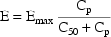
where here  is
understood to mean the prediction of an individual’s
drug concentration in the plasma, and
is
understood to mean the prediction of an individual’s
drug concentration in the plasma, and
 and
and
 are PD (pharmacodynamic
parameters) modeled as
are PD (pharmacodynamic
parameters) modeled as


To fit this data we can use the control
statements of figure 12.1. To obtain initial parameter
estimates, let us assume that the following is observable in
the data. The average value of all effect measurements is
about 50. Across individuals, the average value of the
largest effect measurement within each individual’s
data is about 100, and the average value of the
individual’s observed concentration at about half this
largest measurement is about 20. (This is seen when
concentration measurements and effect measurements are
examined together.) Let us also assume 20% random
interindividual variability in
 and
and
 and 4% intraindividual
variability in the observation. From this we obtain initial
estimates of 100 and 20 for
and 4% intraindividual
variability in the observation. From this we obtain initial
estimates of 100 and 20 for  and
and  ,
,
 for
for
 ,
,
 for
for
 , and
, and
 for
for
 .
.
This example is examined again in in Section 3.2,
which shows the use of $PRED statements, and in Section 5,
which shows how observed concentrations and effects can be
fit simultaneously.
References: Users Guide VI (PREDPP)
IV.B.2
Figure 12.1. The input to NONMEM-PREDPP for analysis of effect observations.
2.2. Other Pharmacokinetic Models: ADVAN5 through ADVAN9
Appendix 1 lists ADVAN routines for the most
commonly-used pharmacokinetic models. Other ADVAN routines
are:
ADVAN5 (General Linear)
ADVAN6 (General Nonlinear)
ADVAN7 (General Linear with Real Eigenvalues)
ADVAN8 (General Nonlinear Kinetics with Stiff Equations)
ADVAN9 (General Nonlinear Kinetics with Equilibrium
Compartments)
With the general methods the user defines a model
of up to 9 compartments using special options of the $MODEL
record. For a linear model (ADVAN5 and ADVAN7), it is
sufficient to specify (directed) compartmental connections
and to compute their rate constant parameters with $PK
statements. ADVAN 5 and 7 make use of numerical
approximations to the matrix exponential. For a nonlinear
model (ADVAN6, ADVAN8, and ADVAN9), differential equations
must be supplied to govern the kinetics, via $DES
statements. For ADVAN9, algebraic equations may also be
supplied via $AES statements. The use of the term
’nonlinear’ with ADVAN 6, 8, and 9 only
indicates that a system of any type of first-order
differential equations is allowed; such equations could be
linear or non-linear.
In all cases, the basic features of PREDPP
described in Chapter 7 are still available, such as the
ability to introduce doses of any kind to any compartment of
the model. It should be noted that the general ADVAN
routines are relatively slow. For example, when a general
method (ADVAN5 or greater) is used for a model identical to
that of an analytic method (ADVAN1 through ADVAN4) the run
time increases, usually by an order of
magnitude.
Some ADVAN and SS routines must be told the
number of accurate digits that are required in the
computation of drug amounts, i.e., the relative tolerance.
This is specified either by the TOL option of the
$SUBROUTINES record or by the $TOL record.
References: Users Guide VI (PREDPP) VI, VII
References: Users Guide IV (NM-TRAN) V.C.3, 4,
7-10
2.3. Zero-Order Bolus Doses
Instantaneous bolus doses, which have AMT>0
and RATE=0, are described in Chapter 6. Such doses appear
instantaneously in the dose compartment. Zero-order bolus
doses are doses that enter the dose compartment via a
zero-order process (in the same manner as do infusions)
except that the rate or duration of the process is computed
with $PK statements. When the RATE data item has the value
-1, then the $PK statements must include an assignment
statement for an additional PK parameter, Rn (the
"modeled rate for compartment n"), whose value
gives the rate of entry of the drug during the interval of
time between the last event record and the current one.
There is a different such parameter for every compartment
receiving a zero-order bolus dose. When the RATE data item
has the value -2, then the $PK statements must include an
assignment statement for an additional PK parameter, Dn (the
"modeled duration for compartment n"), whose value
at the time of the dose event gives the duration time of the
dose. The rate and duration parameters can be modeled like
any other PK parameters; in particular, the assignment
statements can involve  ’s which are to be estimated. These parameters can be
used to model the drug release rate or dissolution time of a
tablet or capsule.
’s which are to be estimated. These parameters can be
used to model the drug release rate or dissolution time of a
tablet or capsule.
Steady-state levels involving zero-order bolus
doses can be computed.
Steady-state with constant infusion was described
in Chapter 6. Steady-state infusions may also have modeled
rates (i.e., the RATE data item may be -1).
References: Users Guide VI (PREDPP) III.F.3,
F.4
2.4. The Additional Dose Data Item: ADDL
ADDL is a dose-related data item that is used to
request that a given number of additional doses, just like
the dose specified on the event record, be added to the
system at a regular time interval, starting from the time on
the event record. PREDPP itself adds these doses at the
appropriate future times; no actual dose event record is
generated by the Data Preprocessor or by PREDPP. A positive
integer value in ADDL specifies how many additional doses
(i.e., in addition to that already specified in the event
record) are to be given, and the value in the II (interdose
interval) data item (which is required) specifies the time
interval between doses.
ADDL may be non-zero on a steady-state dose event
record (except for steady-state infusions), in which case
additional doses are given, maintaining the dosing regimen
into the future. Non-steady-state kinetic formulas are used
to advance the system between each additional dose. See also
Section 2.6 below.
References: Users Guide VI (PREDPP)
V.K
2.5. Lagged doses: the ALAG Parameter
PREDPP permits an additional PK parameter called
an absorption lag time. One such parameter can be defined
for each compartment and applies to all doses to that
compartment. It gives the amount of time that a dose is held
as a "pending" dose. When the absorption lag time
has expired, the dose is input into the system. In effect,
the value of the absorption lag time parameter is added to
the value of the TIME data item on the dose event record.
With NM-TRAN, recognized names for absorption lag time
parameters have the form ALAGn, where n is the compartment
number. See also Section 2.6 below.
References: Users Guide VI (PREDPP) III.F.6
References: Users Guide IV (NM-TRAN) V.C.5
2.6. Controlling Calls to PK and ERROR
In order to evaluate the $PK and $ERROR
statements, PREDPP calls the PK and ERROR subroutines. By
default, the subroutines are called with every event record.
PREDPP may be instructed to limit calls to certain event
records in order to save the computing time involved with
unnecessary calls (e.g. when the PK parameters do not vary
from event record to event record within an individual). It
is also possible to cause the PK subroutine to be called at
times which do not correspond to any actual event
record.
Using NM-TRAN, calls to PK are controlled by the
presence of one of the following pseudo-statements at the
start of the $PK block: call with every event record and at
additional and lagged dose times. call with every event
record (default). call with the first event record of each
individual record and with new values of TIME†.
----------

call once per individual record.
The choice CALLFL=-2 is intended to be
used when PK parameters Dn and/or Fn apply to additional or
lagged doses and the model for these parameters
depends on some time-varying concomitant variable such as
type of drug preparation or patient weight. By default, the
values of the PK parameters which apply to the dose are
those values computed by PK with the first event record
having a value of TIME greater than the time at which the
dose actually enters the system (the additional or lagged
dose time). However, if PREDPP is instructed to also call PK
at the additional or lagged dose time, then the values of
the PK parameters are those values computed at these special
calls. At such calls, PK has available to it information
from the initiating dose event record itself, and
information from the two event records whose TIME values
bracket the additional or lagged dose time. Along with
CALLFL=-2 in the $PK block, the NM-TRAN $BIND
record may be useful; see Users Guide IV.
Using NM-TRAN, calls to ERROR are controlled by
the presence of one of the following pseudo-statements at
the start of the $ERROR block:
call with every event record (default). call with
observation events only†. call once per individual
record.
NM-TRAN automatically instructs PREDPP to limit
calls to ERROR to once per problem for the simple
error models discussed in Chapter 8, Sections 3.1 and
3.2:
Y=F+ERR(1)
Y=F+F*ERR(1)
Y=F*(1+ERR(1))
Y=F*EXP(ERR(1))
During the Simulation Step, PREDPP ignores any
limitation and calls the ERROR subroutine with every event
record.
Even when calls to PK and/or ERROR are limited,
the CALL input data item can be used to force additional
calls for specific event records as needed.
References: Users Guide VI (PREDPP) III.B.2,
III.H, IV.C, V.J
References: Users Guide IV (NM-TRAN) V.C.5, C.6
2.7. Transgeneration of Input Data: the INFN Subroutine
NONMEM may be used to modify the data records
before any computations are performed and also after all
computations have been performed. This is referred to as
transgeneration of the data. Transgeneration at the
beginning of a problem can be used, for example, to change
weight-normalized doses to unnormalized doses. PREDPP allows
the user to supply a subroutine called INFN
("initialization/finalization") in which
transgeneration can be performed. (The PREDPP library
includes a default INFN subroutine which does
nothing.)
References: Users Guide VI (PREDPP)
VI.A
3. User-written PRED Subroutines
It is not necessary to use PREDPP with NONMEM.
Either $PRED statements or a user-written PRED subroutine
may be used in place of PREDPP to supply NONMEM with
predicted values for the DV data item according to some (not
necessarily pharmacokinetic) model. An example using $PRED
statements is given here. A special caveat applies to
user-written PRED subroutines that are recursive: see 4.6
below.
References: Users Guide I (Basic) C.2
3.1. Required Data Items
The only required data items when PREDPP is not
used are the NONMEM data items DV, MDV, and ID. When PREDPP
is used, the Data Preprocessor is able to recognize which
records contain observed values and which do not, and it
supplies the MDV data item if it is not already present in
the data file. When PREDPP is not used, the Data
Preprocessor cannot do this. The input data file must
already contain the MDV data item if it is needed, i.e., if
the DV item of some data record does not contain a value of
an actual observation.
If $PRED statements are used, they must calculate
a variable called Y, using input data items and
NONMEM’s  ,
,
 , and (for population
models)
, and (for population
models)  vectors in the
calculation.
vectors in the
calculation.
References: Users Guide I (Basic) B.1
References: Users Guide IV (NM-TRAN) III.B.8
3.2. An Example of $PRED Statements: Pharmacodynamic Modeling
The syntax of $PRED statements is essentially the
same as discussed for $PK and $ERROR statements. $PRED
statements can be used for simple pharmacokinetic and
pharmacodynamic models. In figure 12.1 above an example was
given of pharmacodynamic modeling using $ERROR statements.
Suppose that in that example, drug concentration is always
measured at the same time as drug effect. Suppose too, that
rather than input the individuals’ values of K and V
and use them to compute a predicted drug concentration for
the individual, the observed drug concentration itself is
used in the Emax model. This means that the the observed
concentrations are again incorporated into the data, but now
as values of an independent variable, rather than as the DV
data item. This also means that a pharmacokinetic model is
not needed, and therefore, PREDPP is not needed either.
Figure 12.2 shows the control stream for this new
example.
Figure 12.2. The input to NONMEM including $PRED statements for analysis of effect data.
4. Advanced Features of NONMEM
4.1. Full Covariance Matrices: $OMEGA BLOCK and $SIGMA BLOCK
In the examples of Chapter 2 and 9, there
appeared statements such as:
$OMEGA .0000055, .04
This is an example of the specification of initial parameter
estimates for a variance-covariance
 matrix which is constrained
to be diagonal. Initial estimates are given for the
variances of
matrix which is constrained
to be diagonal. Initial estimates are given for the
variances of  and of
 . The covariance between
 and
and
 is constrained to be 0,
i.e.,
is constrained to be 0,
i.e.,  . Another way of
writing this statement is:
. Another way of
writing this statement is:
$OMEGA DIAGONAL(2) .0000055, .04
The option DIAGONAL(2) states explicitly that the
block contains two  s and
that it has diagonal form.
s and
that it has diagonal form.
If the data supports the possibility that
 and
and
 covary with each other, it
may be useful to model
covary with each other, it
may be useful to model  as
being unconstrained and allow NONMEM to estimate the
covariance. A special form of the $OMEGA record is used, in
which initial values are supplied for both variances and the
covariance. For example:
as
being unconstrained and allow NONMEM to estimate the
covariance. A special form of the $OMEGA record is used, in
which initial values are supplied for both variances and the
covariance. For example:
$OMEGA BLOCK(2) .0000055, .0000001, .04
The option BLOCK(2) states that there are two
 variables in the block, and
that covariance is to be estimated. The new element is
variables in the block, and
that covariance is to be estimated. The new element is
 .
.
$OMEGA BLOCK is used for both population and
individual studies, i.e., it is the same whether
 is used in the first case
in a model for residual error or is used in the second case
in a model for random interindividual error. In a population
study, if there is more than one
is used in the first case
in a model for residual error or is used in the second case
in a model for random interindividual error. In a population
study, if there is more than one
 variable, and the model
allows these variables to covary, then $SIGMA BLOCK is used
in a similar manner.
variable, and the model
allows these variables to covary, then $SIGMA BLOCK is used
in a similar manner.
The initial estimates of even more complicated
 and
and
 matrices may be given using
multiple $OMEGA and $SIGMA records. For example, the initial
estimates of a mixture of correlated and uncorrelated random
variables may given. Also, in this context (as with the
simple form of the $OMEGA and $SIGMA records described in
Chapter 9, Section 3) variances-covariances may be
constrained to fixed values by means of the FIXED option.
Finally, some variances-covariances may be constrained to
equal others by means of the BLOCK SAME option. The ability
to fix all variances-covariances in both
matrices may be given using
multiple $OMEGA and $SIGMA records. For example, the initial
estimates of a mixture of correlated and uncorrelated random
variables may given. Also, in this context (as with the
simple form of the $OMEGA and $SIGMA records described in
Chapter 9, Section 3) variances-covariances may be
constrained to fixed values by means of the FIXED option.
Finally, some variances-covariances may be constrained to
equal others by means of the BLOCK SAME option. The ability
to fix all variances-covariances in both
 and
and
 allows Bayesian estimates
to be obtained of the pharmacokinetic parameters of a single
individual, based on the individual’s data and a prior
population distribution for the parameters.
allows Bayesian estimates
to be obtained of the pharmacokinetic parameters of a single
individual, based on the individual’s data and a prior
population distribution for the parameters.
References: Users Guide IV (NM-TRAN)
III.B.10
4.2. Grouping Related Observations: The L1 and L2 Data Items
The $ERROR statements for a problem may sometimes
involve more than one random variable. For example, there
may be two types of observations. One type may be an
observation from one compartment of a PK system, or with one
assay or preparation, and another type may be an observation
from a different compartment or with a different assay or
preparation. The model for the two types of observations
would typically involve at least two
 variables (e.g. (3.8)). If
all observations are made at sufficiently separated times,
there may be little reason to be concerned about correlation
between the two random errors. However, if the two types of
observations are taken at the same or very close to the same
time, it is possible that correlation will exist; whatever
circumstance has influenced one observation to be different
from the predicted level may also have some influence on the
other observation. In this case a covariance between the two
variables (e.g. (3.8)). If
all observations are made at sufficiently separated times,
there may be little reason to be concerned about correlation
between the two random errors. However, if the two types of
observations are taken at the same or very close to the same
time, it is possible that correlation will exist; whatever
circumstance has influenced one observation to be different
from the predicted level may also have some influence on the
other observation. In this case a covariance between the two
 variables should be
allowed, as described above in Section 4.1. Then the two
types of observations at the same time point are regarded as
two elements of a multivariate
observation.
variables should be
allowed, as described above in Section 4.1. Then the two
types of observations at the same time point are regarded as
two elements of a multivariate
observation.
In the case of population data, there exists a
NONMEM data item, L2, which is used to identify the elements
of a multivariate observation. In effect, L2 acts in a
similar way as ID, but grouping observations within
individual records.
In the case of individual data, the ID data item
already serves this purpose: it forms groups of observations
whose  variables may be
correlated. Thus, in the input data file, the ID data item
should be the same for those observations which may have
correlated
variables may be
correlated. Thus, in the input data file, the ID data item
should be the same for those observations which may have
correlated  s. However, for
individual data, the Data Preprocessor normally replaces the
ID data item with a new set of values which describe every
observation as being independent of the others. To prevent
the Data Preprocessor from doing this, L1 should be included
in the $INPUT record as the name or synonym for the
user-supplied ID data item.
s. However, for
individual data, the Data Preprocessor normally replaces the
ID data item with a new set of values which describe every
observation as being independent of the others. To prevent
the Data Preprocessor from doing this, L1 should be included
in the $INPUT record as the name or synonym for the
user-supplied ID data item.
References: Users Guide IV (NM-TRAN) II.C.4,
III.B.2
References: Users Guide II (Supplemental) D.3
4.3. Continuing a NONMEM Run: MSFO and MSFI
The MSFO (Model Specification Output
File) option of the $ESTIMATION record instructs NONMEM to
write a Model Specification File (MSF) when the
Estimation Step finishes. This file can then be read in a
subsequent NONMEM run using a $MSFI (Model Specification
File Input) record. This file has much of the information
about the model used in the previous run, thus the name
"Model Specification File". It also contains all
the information that allows the Estimation Step from the
previous run (which may have terminated, for example, due to
the number of function evaluations exceeding its limit) to
be continued in the subsequent run. There are a number of
benefits to using a MSF. First, what might be a long
Estimation Step (due to a very lengthy search) can be split
over a series of runs, each with a limited number of
function evaluations. Any run which terminates prematurely
due to computer failure can be restarted from the MSF output
in the previous run. (This provides a
"checkpoint/restart" capability.) The progress
made in the Estimation Step can also be evaluated between
runs, and a decision made as to whether it is worth
continuing a search which is consuming excessive amounts of
computer time. Second, the Covariance, Tables, and
Scatterplot Steps can be performed in later runs, each using
the MSF from the final run with the Estimation Step. It is
advisable to perform the Covariance Step only after
satisfactory results have been obtained from the Estimation
Step.
References: Users Guide I (Basic) C.4.4
References: Users Guide IV (NM-TRAN) III.B.6,
B.12
4.4. NONMEM Can Obtain Initial Estimates for , ,
NONMEM can be directed to obtain initial
estimates for one or more elements of
 ,
,
 , or
, or
 . This is done in a
separate Initial Estimates Step. For an element of
. This is done in a
separate Initial Estimates Step. For an element of
 , omit the initial estimate
but include lower and upper bounds, e.g., (1, ,50) in the
$THETA record. (The NUMBERPOINTS option may be used to
control the number of points in
, omit the initial estimate
but include lower and upper bounds, e.g., (1, ,50) in the
$THETA record. (The NUMBERPOINTS option may be used to
control the number of points in
 space examined by NONMEM
during the search for initial estimates of
space examined by NONMEM
during the search for initial estimates of
 .) For a block of
 or
or
 , omit all initial
estimates on the $OMEGA BLOCK (or DIAGONAL) record, or
$SIGMA BLOCK (or DIAGONAL) record, respectively.
, omit all initial
estimates on the $OMEGA BLOCK (or DIAGONAL) record, or
$SIGMA BLOCK (or DIAGONAL) record, respectively.
Note that when $PK and $ERROR statements are
present but the $OMEGA and/or $SIGMA records are absent,
NONMEM will be directed to obtain initial estimates for the
variances of the random variables in question, assuming the
diagonal form of the matrix.
References: Users Guide IV (NM-TRAN)
III.B.9-11
4.5. Improving Parameter Estimates: REPEAT and RESCALE
The Estimation Step can be immediately repeated
after the search has terminated successfully, by including
the REPEAT option on the $ESTIMATION record. This
can improve the accuracy of the parameter estimates when one
or more initial estimates are wrong by a few orders of
magnitude. The final estimates from the first implementation
of the Estimation Step are used as the initial estimates of
the second implementation, and thus the scaling used with
the STP is different from that with the first
implementation, allowing fewer leading zeros after the
decimal point in the STP. When the Estimation Step is
continued by means of a Model Specification File, similar
rescaling can be requested using the RESCALE option
of the $MSFI record.
References: Users Guide IV (NM-TRAN) III.B.12,
B.14
References: Users Guide II (Supplemental) F
4.6. The Covariance Step: , , Special Computation
The Covariance Step, which computes standard
errors of the parameter estimates, first computes a
covariance matrix of the parameter estimates. (This is not
the same as the  or
or
 matrix). It is possible to
request that this covariance matrix be computed in one of
three different ways: either as
matrix). It is possible to
request that this covariance matrix be computed in one of
three different ways: either as
 ,
,
 , or
, or
 (the default), where
 and
and
 are two matrices from
statistical theory, the Hessian and Cross-Product Gradient
matrices, respectively. Options MATRIX=R and
MATRIX=S of the $COVARIANCE record are used to
request the
are two matrices from
statistical theory, the Hessian and Cross-Product Gradient
matrices, respectively. Options MATRIX=R and
MATRIX=S of the $COVARIANCE record are used to
request the  and
and
 matrices, respectively. The
Covariance Step can produce additional output. When the
default covariance matrix is used,
matrices, respectively. The
Covariance Step can produce additional output. When the
default covariance matrix is used,
 and/or
 can be printed. This is
requested by options PRINT=R and/or
PRINT=S. Eigenvalues are be printed if requested by
option PRINT=E. Multiple PRINT options can
be specified.
can be printed. This is
requested by options PRINT=R and/or
PRINT=S. Eigenvalues are be printed if requested by
option PRINT=E. Multiple PRINT options can
be specified.
A special computation is required when the
data are from a single individual and a recursive PRED is
used. A recursive PRED is one which stores the results of
certain computations using the values from one event record,
and uses these results in later computations with the values
from a later event record. PREDPP advances the kinetic
system from one time point to the next and therefore is an
example of a recursive PRED. When PREDPP is used and the
data is from a single individual, NM-TRAN automatically
requests the special computation. When a recursive
user-written PRED is used and the data are from a single
individual, the SPECIAL option of the $COVARIANCE
record must be used.
The CONDITIONAL option of the
$COVARIANCE record requests that the Covariance Step be
implemented only if Estimation Step terminates successfully,
and is the default. The UNCONDITIONAL option can be
used to request that it be implemented no matter how the
Estimation Step terminates.
References: Users Guide IV (NM-TRAN) III.B.15
References: Users Guide II (Supplemental) D.2.5
4.7. Multiple Problems in a Single NONMEM Run
NONMEM can implement more than one problem in a
single run. That is, the input control stream can contain
more than one $PROBLEM record, each followed by its own set
of problem specification statements. This feature can be
useful in a variety of situations. A series of what
otherwise would be separate runs, each analyzing a single
individual’s data within a population data file, can
be performed conveniently without building separate data
files for each individual. Also, more than one data set can
be analyzed using the same model and the same problem
specification. Multiple problems are also useful with
NONMEM’s Simulation Step, described below.
Note that $PK and $ERROR statements cannot appear
after the first problem, even when the PK and ERROR
subroutines from the PREDPP library are used. This is a
restriction in NM-TRAN Version II. If the $DATA record is
omitted or the filename is specified as * on a $DATA record
in a problem subsequent to the first, the previous data set
is re-used.
References: Users Guide IV (NM-TRAN)
III.B.1
4.8. Simulation Using NONMEM: The $SIMULATION Record
The term simulation refers to the
generation of data points according to some model. A simple
form of simulation is performed when the Estimation Step is
omitted but the Table Step is implemented. The PRED column
of the table contains predictions based on the information
in the data records and the initial estimates of
 , under the model specified
in the PRED (PREDPP) subroutine. Random variables
, under the model specified
in the PRED (PREDPP) subroutine. Random variables
 and
and
 (if any) have no effect on
the predictions and may be omitted. If the only purpose of
the run is to obtain simulated values, and these variables
are present, it is best (but not required) that their
variances be fixed to 0. NONMEM does not compute the
objective function in this circumstance, which has certain
advantages.
(if any) have no effect on
the predictions and may be omitted. If the only purpose of
the run is to obtain simulated values, and these variables
are present, it is best (but not required) that their
variances be fixed to 0. NONMEM does not compute the
objective function in this circumstance, which has certain
advantages.
NONMEM can also perform a Simulation Step, in
which another type of simulation is performed. In the
Simulation Step, each value of the DV data item of each
record with MDV=0 is replaced by a simulated observation
generated from the model, but including statistical
variability†.
----------

The PRED (PREDPP) routine uses
 and
and
 values that are supplied by
NONMEM according to user-specified random distributions
(e.g., with variances given by the initial estimates of
values that are supplied by
NONMEM according to user-specified random distributions
(e.g., with variances given by the initial estimates of
 and
and
 ). If
). If
 and
and
 matrices are fixed to zero,
for example, the simulated values are the same as the
predictions described above.
matrices are fixed to zero,
for example, the simulated values are the same as the
predictions described above.
If the data are then displayed by the Table Step,
the DV column for records with MDV=0 contains the simulated
observations obtained from the Simulation Step. For records
having MDV=1, the DV column contains whatever was in the
original data record. The PRED column of the table contains
predictions as described above. If the Estimation Step was
not implemented, the values of
 used for these predictions
are the initial values. If the Estimation Step was
implemented, the values of
used for these predictions
are the initial values. If the Estimation Step was
implemented, the values of  used for the predictions in the PRED column are the final
parameter estimates. Note that the observations that are fit
during the search are the simulated values obtained by the
Simulation Step.
used for the predictions in the PRED column are the final
parameter estimates. Note that the observations that are fit
during the search are the simulated values obtained by the
Simulation Step.
Often data are simulated using the Simulation
Step, then analyzed using one or more other steps (e.g.
Estimation and Covariance Steps), and this process is
repeated a fixed number of times, using the same model. The
Simulation Step accommodates this easily with the notion of
a NONMEM subproblem, whereby these steps are repeated
within the same NONMEM problem. However, on occasion it can
be useful to have multiple problems (see Section 4.7), where
one problem implements the Simulation Step, and the
subsequent problem implements other steps. For example, this
is one way to obtain different initial parameter estimates
for the Estimation Step than for the Simulation
Step.
The ONLYSIMULATION option causes NONMEM
to suppress evaluation of the objective function. With this
option, PRED-defined variables displayed in tables and
scatterplots (see Section 4.13) are simulated values, i.e.,
use simulated  s and initial
 s, and weighted residual
values in tables and scatterplots are always 0.
s, and weighted residual
values in tables and scatterplots are always 0.
References: Users Guide IV (NM-TRAN) III.B.13
References: Users Guide VI (PREDPP) III.E.2, L.1 , IV.B.1-2,
C, G.1
4.9. Files for Subsequent Processing: the $TABLE Record
NONMEM can write the data for a table to an
external formatted file, as requested by the FILE option of
the $TABLE record. Other computer programs can read these
files. Such programs can perform further analysis or provide
improved graphical displays. These files normally contain
header lines similar to those in a printed table, but the
header lines can be suppressed entirely or in part by means
of the NOHEADER or ONEHEADER options,
respectively.
References: Users Guide IV (NM-TRAN)
III.B.16
4.10. Data Checkout Mode
NONMEM’s data checkout mode is intended for
preliminary display of data without the use of a model. In
data checkout mode, the PRED routine is not called.
Predictions, the objective function, residuals, and weighted
residuals are not computed. Only the Table and Scatterplot
Steps can be implemented in the problem. With NM-TRAN, this
mode is requested by coding the option CHECKOUT on
the $DATA record. A $SUBROUTINES record and abbreviated code
are required, but they have no effect and need only be
syntactically correct.
References: Users Guide IV (NM-TRAN)
III.B.6
4.11. Obtaining Individual Parameter Estimates - Conditional Estimates of s
With population data, NONMEM can obtain estimates
of individual-specific true values of
 from any given set of
values of
from any given set of
values of  ,
,
 ,
,
 , and the
individual’s data. These are called conditional
estimates of
, and the
individual’s data. These are called conditional
estimates of  . When the
conditional estimates are obtained after estimation is
carried out by the First-Order method, they are referred to
as "posthoc" estimates. With NM-TRAN, they are
requested by the option POSTHOC on the $ESTIMATION
record.
. When the
conditional estimates are obtained after estimation is
carried out by the First-Order method, they are referred to
as "posthoc" estimates. With NM-TRAN, they are
requested by the option POSTHOC on the $ESTIMATION
record.
References: Users Guide IV (NM-TRAN)
III.B.14
4.12. Population Conditional Estimation Methods
NONMEM can obtain conditional estimates of
 variables as part of the
computation of population parameter estimates. These are
called conditional estimation methods. With NM-TRAN,
such methods are requested by including the option
METHOD=CONDITIONAL (or METHOD=1) on the
$ESTIMATION record. (The option METHOD=ZERO, or
METHOD=0, requests the conventional First-Order
method and is the default.) There are two conditional
estimation methods. If NONMEM uses only first-order
approximations, this is the First-Order Conditional
Estimation Method. This has one variation,
interaction, which takes into account
variables as part of the
computation of population parameter estimates. These are
called conditional estimation methods. With NM-TRAN,
such methods are requested by including the option
METHOD=CONDITIONAL (or METHOD=1) on the
$ESTIMATION record. (The option METHOD=ZERO, or
METHOD=0, requests the conventional First-Order
method and is the default.) There are two conditional
estimation methods. If NONMEM uses only first-order
approximations, this is the First-Order Conditional
Estimation Method. This has one variation,
interaction, which takes into account
 -
-
 interaction and is
requested by the additional option INTERACTION on
the $ESTIMATION record. If NONMEM uses a certain
second-order approximation, this is the Laplacian
method, which is requested by the additional option
LAPLACIAN on the $ESTIMATION record. Interaction
cannot be specified with the Laplacian method.
interaction and is
requested by the additional option INTERACTION on
the $ESTIMATION record. If NONMEM uses a certain
second-order approximation, this is the Laplacian
method, which is requested by the additional option
LAPLACIAN on the $ESTIMATION record. Interaction
cannot be specified with the Laplacian method.
Note that this usage of the term CONDITIONAL is
different from the usage on the $SCATTERPLOT, $TABLE, and
$COVARIANCE records, in which it refers to the circumstances
under which the step in question is implemented.
References: Users Guide IV (NM-TRAN)
III.B.14
4.13. Displaying PRED-Defined Variables and Conditional Estimates of s
NONMEM can display PRED-defined variables in
table and scatterplots. With NM-TRAN, any variable appearing
on the left-hand side of an assignment statement in
abbreviated code can be displayed by listing it in a $TABLE
or $SCATTER record. If the data are population, NONMEM can
also display conditional estimates of
 . With NM-TRAN, variables
ETA(1), ETA(2), etc., can be simply listed in $TABLE and
$SCATTER records. When conditional estimation is not
performed, the values displayed are zero. Displayed values
of PRED-defined true-value variables will use conditional
estimates of
. With NM-TRAN, variables
ETA(1), ETA(2), etc., can be simply listed in $TABLE and
$SCATTER records. When conditional estimation is not
performed, the values displayed are zero. Displayed values
of PRED-defined true-value variables will use conditional
estimates of  if they have
been obtained, otherwise they will be typical values. This
feature is available with PREDPP, as well as with
user-written PRED routines. For example, the following
records could replace the $ESTIMATION record in Figure
12.2:
if they have
been obtained, otherwise they will be typical values. This
feature is available with PREDPP, as well as with
user-written PRED routines. For example, the following
records could replace the $ESTIMATION record in Figure
12.2:
$ESTIMATION POSTHOC
$TABLE ETA(1) EMAX
The $ABBREVIATED record can be used to limit the
number of variables available for display when the number is
excessive.
References: Guide III (Installation) V.2.4
References: Guide IV (NM-TRAN) III.B.16-17
References: Guide VI (PREDPP) III.J, IV.E
4.14. Mixture Models
A mixture model is a model that explicitly
assumes that the population consists of two or more
sub-populations, each having its own model. For example,
with two sub-populations, one might assume that some
fraction p of the population has one set of typical values
of the PK parameters, and the remaining fraction 1-p has
another set of typical values. Both sets of typical values
and the mixing fraction p may be estimated. For each
individual, NONMEM also computes an estimate of the number
of the subpopulation of which the individual is a member.
The user must supply a FORTRAN subroutine called MIX to
compute the fractions p and 1-p.
References: Users Guide VI (PREDPP)
III.L.2
4.15. PRED Error Return Codes and Error Messages in File PRDERR
A PRED routine can return a PRED error return
code (1 or 2) to NONMEM, indicating that it is unable to
compute a prediction for a given data record with the
current values of  ’s
and
’s
and  ’s. For example,
PREDPP returns error return code 1 when a basic or
additional PK parameter has a value that is physically
impossible (e.g., a scale parameter which is zero or
negative). Error return codes can also be specified by the
user in user-written code or in abbreviated code using the
EXIT statement. One reason for doing this is to constrain
parameters in order to avoid floating point machine
interrupts. The PRED error recovery option determines
what action NONMEM will take. With NM-TRAN, the PRED error
recovery option is either ABORT (which is the
default) or NOABORT, and is specified on the
$ESTIMATION and $THETA records.
’s. For example,
PREDPP returns error return code 1 when a basic or
additional PK parameter has a value that is physically
impossible (e.g., a scale parameter which is zero or
negative). Error return codes can also be specified by the
user in user-written code or in abbreviated code using the
EXIT statement. One reason for doing this is to constrain
parameters in order to avoid floating point machine
interrupts. The PRED error recovery option determines
what action NONMEM will take. With NM-TRAN, the PRED error
recovery option is either ABORT (which is the
default) or NOABORT, and is specified on the
$ESTIMATION and $THETA records.
If an error return code is returned during the
Simulation, Covariance, Table or Scatterplot Step, or during
computation of the initial value of the objective function,
NONMEM will abort. If the error return code is returned
during the Estimation or Initial Estimates Step, NONMEM will
try to avoid those values of
 and
and
 for which the error
occurs. If they cannot be avoided, NONMEM’s actions
depend on the error return code value, as
follows:
for which the error
occurs. If they cannot be avoided, NONMEM’s actions
depend on the error return code value, as
follows:
|
1
|
|
If NOABORT is specified on $ESTIM or
$THETA, try to avoid the current values of
 and and
 . If ABORT is
specified on $ESTIM or $THETA, then abort. . If ABORT is
specified on $ESTIM or $THETA, then abort.
|
PRED routines may optionally provide text
accompanying the error return code. NONMEM writes all text
associated with error return codes to a file, PRDERR. The
contents of this file should always be carefully
reviewed.
References: Users Guide III (Installation)
III.2.1.1
References: Users Guide IV (NM-TRAN) IV.A, IV.C.5-6
References: Users Guide VI (PREDPP) III.K, IV.F
4.16. User-Written Subroutines
Although most NONMEM applications can be
accomplished using NM-TRAN abbreviated code, there are cases
in which user-written FORTRAN subroutines are needed. The
$SUBROUTINES record allows the user to specify the
names of user-written routines that are needed in the NONMEM
load module. A user may choose to write his own PRED, PK,
ERROR, MODEL, DES, or AES subroutine. Some subroutines that
are distributed with NONMEM are dummy, or "stub"
routines, that do nothing. Of these, subroutines CCONTR,
CONPAR, CONTR, and CRIT can be replaced to obtain an
objective function different from the default. NONMEM
subroutine MIX must be replaced for mixture models. PREDPP
subroutine INFN may be replaced by user-written code. The
names of all such routines are specified using the
identically named options of the $SUBROUTINES
record, e.g., PRED=subname, CONTR=subname,
etc. User-written routines may call other FORTRAN
subroutines, which can be specified for inclusion in the
load module using the option
OTHER=subname.
With user-written CONTR routines, the NM-TRAN
$CONTR record may be useful.
References: Users Guide IV (NM-TRAN) III.B.4,
B.6
5. Observations of Two Different Types
An NM-TRAN control stream is shown in Figure
12.3, for the analysis of a data set which contains
observations of two different types. A fragment of the data
set, shown in Figure 12.4, contains the data for one
individual. This example illustrates how concentration and
effect data can be fit simultaneously, and includes many of
the advanced features described in this chapter, such as
pharmacodynamic modeling in the $ERROR statements,
correlation between elements of
 , and the L2 data
item.
, and the L2 data
item.
Suppose that the data set for the phenobarbital
example of Chapter 2 is modified to include both
concentration and effect observations, and that a data item
called TYPE is used to distinguish between them. When TYPE
is 1, DV contains an effect measurement. When TYPE is 2, DV
contains a concentration. The $PK statements are the same as
those of Figure 2.12. The $ERROR statements are the same as
those of Figure 12.1, except that the elements of
 and
and
 are renumbered to follow
those used in the $PK statements. The (true-value) variable
Y1 is assigned the same value as Y in the $ERROR statements
of Figure 12.1 The (true-value) variable Y2 is assigned the
same value as Y in the $ERROR statements of Figure 2.12,
except that
are renumbered to follow
those used in the $PK statements. The (true-value) variable
Y1 is assigned the same value as Y in the $ERROR statements
of Figure 12.1 The (true-value) variable Y2 is assigned the
same value as Y in the $ERROR statements of Figure 2.12,
except that  is used rather
than
is used rather
than  .
.
The input data file contains observations of both
types which were made at the same time value. The event
records therefore include the L2 data item. Figure 12.4,
like Figure 2.7, shows the data for the first individual,
but includes TYPE and L2 data items and effect observations.
Note that the L2 data item has a different value for each
multivariate observation within the individual record. (The
values 1 and 2 are chosen arbitrarily and may be re-used for
the L2 data items in the next individual’s data, if
desired.)
The $THETA, $OMEGA, and $SIGMA records contain
the values shown in Figures 2.12 and 12.1 and one other
value, 2.8, for the covariance
 . The estimate 2.8 is
chosen so that the correlation is, arbitrarily, .5 (
. The estimate 2.8 is
chosen so that the correlation is, arbitrarily, .5 (
 ).
).
Figure 12.3. The input to NONMEM-PREDPP for analysis of the population phenobarbital data, including both concentration and effect observations.
Figure 12.4. The first individual's phenobarbital data, including both concentration and effect observations.
TOP
TABLE OF CONTENTS
NEXT