NONMEM Users Guide Part V - Introductory Guide - Chapter 7

Chapter 7 - $SUBROUTINE Record and $PK Record

1. What This Chapter is About

This chapter tells how to write a $SUBROUTINE record and how to write a simple $PK record for both individual and population data. This chapter is meant to be read in parallel with Chapters 3 and 4.

2. The $SUBROUTINE Record

The $SUBROUTINE record describes which pharmacokinetic model is to be used. Recall that NONMEM calls a subroutine named PRED to compute the predicted value. The user must choose to use his own PRED subroutine or to use the PREDPP package. In this text it is assumed that the PREDPP package is chosen.

2.1. Choosing an ADVAN Subroutine: Standard Pharmacokinetic Models

The PREDPP Library includes five subroutines which are pre-preprogrammed, each for a specific pharmacokinetic model. They are:
ADVAN1 (One Compartment Linear Model)
ADVAN2 (One Compartment Linear Model with First Order Absorption)
ADVAN3 (Two Compartment Linear Model)
ADVAN4 (Two Compartment Linear Model with First Order Absorption)
ADVAN10 (One Compartment Model with Michaelis-Menten Elimination)
PREDPP calls only one subroutine, ADVAN; the different names above are external names distinguishing different instances of the ADVAN routine in the PREDPP Library. The name ’ADVAN’ is used because the routine advances (i.e. updates the state of) the kinetic system from one point in time to the next. There are additional ADVAN routines in the Library which implement more general types of pharmacokinetic models; see Chapter 12, Section 2.2. Each of the ADVAN’s can be used for either individual or population data. The (external) name of the ADVAN to be used is coded on the $SUBROUTINE record; this also implies that PREDPP is to be used.
----------

As an example, the following record specifies the One Compartment Linear Model:
$SUBROUTINE ADVAN1

The five ADVAN’s are described in Appendix 1. They share certain features.

On event records, the output compartment is referred to by the compartment number given in Appendix 1. A PK parameter which refers to the output compartment may use either this number or 0 (zero). Thus, F0 and F2 both denote the output fraction for ADVAN1; similarly, S0 and S4 both denote the scale for ADVAN4’s output compartment.

2.2. Choosing a TRANS Subroutine: Alternative Parameterizations

As discussed in Chapter 3, we may prefer to use pharmacokinetic parameters in our PK routine other than the microconstants used by PREDPP. Appendix 2 shows several commonly-used parameterizations. The PREDPP package includes a family of subroutines called TRANS routines which are pre-programmed to translate (reparameterize) from these commonly used parameterizations to the ones expected by PREDPP. Appendix 2 also gives the TRANS routine for each alternative parameterization. As with ADVAN, TRANS is the name of the routine. The names given in Appendix 2 are instances of external subroutine names used in the PREDPP Library. The first member of the family, TRANS1, simply translates a set of microconstants into these same microconstants and must be included in the NONMEM load module in lieu of the others when the $PK abbreviated code computes the microconstants.

The user must describe on the $SUBROUTINE record which TRANS routine is to be used. For example, the following record requests the One Compartment Linear Model parameterized (in the PK routine) in terms of clearance and volume.
$SUBROUTINE ADVAN1,TRANS2
When a TRANS other than TRANS1 is used, only the alternative parameters listed in column 1 need be assigned values in the $PK abbreviated code. In this example, these are CL, V, and KA.

Note that TRANS1 is the default. That is, if no TRANS routine is listed on the $SUBROUTINE record, it is assumed that TRANS1 is intended. This is the case in the examples of Chapter 2. Alternative parameterizations using TRANS1 are discussed later in this chapter in Section 4.2.

2.3. Other Options

The $SUBROUTINE record also describes how the abbreviated code is to be implemented, as discussed in Section 3 of Chapter 1. The choices are: DOUBLE (double-precision FORTRAN subroutines), SINGLE (single-precision FORTRAN subroutines), or LIBRARY (library subroutines whose precision is chosen at the time the NONMEM-PREDPP load module is built). The default is DOUBLE. Thus, the following two records are equivalent:
$SUBROUTINE ADVAN1,TRANS2
$SUBROUTINE ADVAN1,TRANS2 DOUBLE

3. $PK Abbreviated Code

$PK abbreviated code consists of a block of $PK statements, one per line, which look much like FORTRAN77 statements. In fact, they are a subset of FORTRAN77: simple assignment statements and certain kinds of conditional (IF) statements. The $PK abbreviated code must be preceded by a record containing the characters "$PK". This record and the abbreviated code constitute the $PK record.

$PK statements must include assignment statements giving a value to every basic PK parameter for the given ADVAN and TRANS combination, as listed in Appendix 1 (when TRANS1 is used) or column 1 of Appendix 2 (when a different TRANS is used). They may also include assignment statements giving values to one or more of the additional PK parameters.

3.1. Syntax

We assume the readers of this document are familiar with writing FORTRAN assignment and conditional statements. If not, the examples in this and the following chapter should give adequate guidance. FORTRAN statement numbers are not used, and the statements may start in any column. As with all NM-TRAN records, blank lines are permitted, and all text following a semi-colon (;) is ignored and may be used for comments. FORTRAN continuation lines are not permitted.

The statements are built using the following: elements of the THETA array (e.g., THETA(1)); constants; names of input data items appearing on the $INPUT record; names of previously-assigned variables; FORTRAN library functions SQRT, LOG, LOG10, and EXP; arithmetic operators +, -, *, /, **; and arithmetical and logical expressions using all of the above. In addition, statements may include representations for random variables such as ETA(1) and EPS(3). Input data items have the values appearing on the current event record, and thus these values may change from one event record to the next. A user-defined variable name follows the usual FORTRAN rules (1-6 letters and digits, starting with a letter) and may not be subscripted. It is defined ("declared") by being assigned a value (i.e., by appearing to the left of = in an assignment statment).

Neither nested parentheses nor nested IF statements are allowed, but this restriction can be avoided by the use of user-defined variables. Moreover, a pair of parentheses enclosing a subscript may be nested within another pair of parentheses. All subscripts must be constants (e.g. THETA(1)). The statements are evaluated sequentially, in the order in which they appear.

All variables, constants, and expressions are evaluated using floating-point (not integer) arithmetic. Single or double precision function names and constants may be used interchangeably. The choice of single precision versus double precision is made on the $SUBROUTINES record and overrides the apparent precision of the statements.

3.2. When are $PK Statements Evaluated?

$PK statements are normally evaluated with every event record for both population and individual data†. This enables the amounts in the compartments to be updated from event time to event time using current values of the data items.
----------

This may be more frequent than is necessary. In the theophylline example of Chapter 2, no data item is used in the $PK statements. In the phenobarbital example, the data item used, WT, is constant within any individual’s data. In these cases, it is sufficient, and it can save noticeable amounts of run time, to evaluate the $PK statements once per individual record. PREDPP can be instructed that the set of event records with which the $PK statements are evaluated are to be limited in some way (see Chapter 12, Section 2.6). The CALL data item can be used to force the statements to be evaluated with any event records.

Certain advanced forms of dosing (additional and lagged doses; see Chapter 12, Sections 2.4 and 2.5) introduce doses at times which do not necessarily coincide with any event record. PREDPP does not normally evaluate the $PK statements at such times, but can be instructed to do so (Chapter 12, Section 2.6).

3.3. Time Varying PK parameters

The state of the kinetic system at a given event time is obtained using PK parameter values computed with the data items on the event record. Using these parameter values the system is advanced to the event time from the last event time. Population models sometimes use data items which change value within individual records and thus give

rise to PK parameters whose values change within individual records. In Chapter 4, Section 3.1.6, it is pointed out that it is desirable for the value of such a data item on the event record to be that value holding at the midpoint of the interval between the current event time and the last previous event time, since the system is advanced over this interval using the PK parameters determined with this value.

If the data item changes too rapidly for this value to fairly represent the data item over the entire time period, it is possible to subdivide the interval into smaller intervals. Event records with EVID=2 (other type event records) can be introduced for this purpose. For example, between two consecutive event records and , with event times and , one might introduce two new other type event records and , with event times and , into the data set. The value of the data item in will be used to compute the PK parameters used to advance the system over the interval to and should be the value of the data item holding at the midpoint of this interval. Similarly, the value of the data item in will be used to compute the PK parameters used to advance the system over the interval to and should be the value of the data item holding at the midpoint of this interval, and so on.

4. $PK Statements for Individual Data

4.1. Basic and Additional Parameters

With individual data, the parameters to be estimated are (usually) the individual’s PK parameters, and therefore, elements of should be associated with these PK parameters. (NONMEM estimates the elements of the vector.) By an individual’s PK parameters, we mean here the basic PK parameters and, possibly, some additional PK parameters (e.g. a bioavailability fraction, or volume of distribution when the latter is not a basic PK parameter). To illustrate, in the theophylline example of Chapter 1 there occur these $PK statements
$PK
KA=THETA(1)
K=THETA(2)
The parameters KA and K are the basic PK parameters for ADVAN2 and TRANS1 (the default TRANS routine). They are used to compute the amounts in the compartments. Typically, however, the observations are concentrations. A scale parameter is used to convert the amount into a concentration. Thus, in the theophylline example we see two additional $PK statements:
V=THETA(3)
S2=V
Here, V is a user-defined variable standing for the volume of distribution of the central compartment. It is neither a basic nor additional parameter. The parameter S2 is the scale parameter for the central compartment; upon dividing the amount in that compartment by S2, the concentration results. (An observation is usually predicted by an amount for a compartment divided by that compartment’s scale parameter). In fact, these two statements could be replaced by the single statement
S2=THETA(3)
However, it may be helpful to the user to distinguish in his code between the calculation of the central volume itself and the calculation of the scale parameter.

There is no particular need for certain elements of to be associated with certain PK parameters. In the above example, the roles of and could have been reversed. NONMEM’s vector may contain more or fewer elements than there are PK parameters, depending on how these parameters are modeled.

PK parameters must be explicitly modeled, usually in terms of parameters to be estimated and user-defined data items; the user communicates this model with the $PK statements. If a certain parameter’s value is known a priori (say, S2 has the known value 500), there are several ways the value can be incorporated into the $PK statements. The following examples show how it can be done via a constant, via a fixed element of , and via a (differently-named) data item:

4.2. Alternative Parameterizations using $PK Statements

It is possible to use an alternative parameterization while still using TRANS1. The reparameterization is performed within the $PK statements by explicitly computing the microconstants from the alternative parameters. Such "reparameterization" statements are given in column 2 of Appendix 2. They must follow the assignment statements that give the alternative parameters their values, as in the phenobarbital example of Chapter 2.

The advantage of using $PK statements to reparameterize, rather than using a TRANS subroutine, is that the NONMEM-PREDPP load module will then always consist of the same set of subroutines for a given choice of ADVAN, which simplifies the job of creating and running it. It will also run slightly faster. We assume in this document that this approach is taken.

Other parameterizations are possible besides the ones in Appendix 2. For example, with ADVAN1 and TRANS1, one might code:
CL=THETA(1)
K=THETA(2)
V=CL/K
S1=V

The ability to express a large variety of modeling possibilities with NONMEM-PREDPP provides great freedom and flexibility, but as always with flexible modeling capability, certain pitfalls arise. Suppose, for example, that with a one compartment system the compartment amount, rather than the concentration is observed. With ADVAN1 and TRANS1 the statements
CL=THETA(1)
V=THETA(2)
K=CL/V
will lead to difficulty because only the ratio of to affects the amount in the compartment, and therefore, the data do not allow and to be separately estimated. The statements should read:
K=THETA(1)

It is important to remember that only those elements of which affect the predictions of observations will be estimated by NONMEM. Here is some problematic code using ADVAN1 with TRANS1:
K=THETA(1)
V=THETA(2)
CL=THETA(3)
S1=V
Once again, NONMEM will be unable to produce separate estimates of all elements of . The kinetics of a simple one compartment system cannot be determined by three independent parameters. With TRANS1, PREDPP itself does not "know" about the relationship K=CL/V which defines a dependency among the parameters. Indeed, the parameters CL and V are both regarded as user-defined variables. The value of has no effect on the prediction. Were it not for the fact that S1 is set equal to V, the value of would have no effect on the prediction either. With TRANS2 this code is also incorrect for essentially the same reason. Here, K is regarded as a user-defined variable, and the relationship CL=K*V is not "known" to PREDPP. (PREDPP does know that CL/V is the rate constant of elimination, but it does not recognize the variable K as denoting this rate constant, and has no effect on the prediction.)

4.3. Scale Parameters

Scale parameters are mentioned in Section 2.1. Predicted compartment amounts are divided by them and are thus converted to predicted concentrations. They are only needed for those compartments whose concentrations are directly observed. With ADVAN3, for example, the peripheral compartment’s scale S2 does need to be computed explicitly if there are no observation events giving measured values of concentrations in the peripheral compartment. Predicted values for this compartment may still be plotted against time, for example, but these values need not be scaled drug amounts; the (unscaled) amount alone is sufficient to show the shape of the curve. (The various volume parameters shown in Appendix 2 must be modeled when they are used as basic parameters, but they need not be assigned as values to compartment scale parameters.) Any scale parameter which is not modeled by $PK statements is assumed to be 1 (i.e., predicted values are always amounts).

4.3.1. Scaling by a Known Constant

In Chapter 3, Section 2.2.1, the units of V were changed from kiloliters to liters using the model:

This can be coded in a $PK statement similar to the way it appears here, except that the compartment number must be specified:
S1=V/1000
Basic PK parameters may also be rescaled in this manner.

4.3.2. Scaling by a Parameter: Conditional Statements and Indicator Variables

In Chapter 3, Section 2.2.2, the following model appeared:

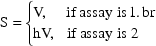
There are two ways this can be coded in $PK statements. The data item can be tested directly, or an indicator variable can be used. An indicator variable is a variable whose value is 0 or 1. It may be identified with an input data item, or it may be a user-defined variable in the $PK statements. For example, suppose variable ASY is to be used as an indicator variable. If some input data item is given value 1 when assay 1 was used and value 0 when assay 2 was used, then this data item could simply be named ASY on the $INPUT record. Suppose, however, that the assay number itself (1 or 2) was recorded in the data and that we have named the data item ANUM on the $INPUT record. We must compute the user-defined variable ASY for use as an indicator variable. There are two ways this can be done: using a logical IF and using a block IF.

The choice between these forms of IF is purely a matter of style. Now let us assume that the compartment to be scaled is compartment 2, and that is to be identified with . The parameter S2 can now be coded unconditionally:
S2=ASY*V+(1-ASY)*THETA(5)*V

Alternatively, ANUM can be tested and ASY avoided altogether:

4.3.3. Scaling by a Data Item

If observations of urine concentration are included in the data (see e.g. Chapter 6, Section 9), it is necessary to provide urine volume as a scale for the output compartment. Presumably, this volume varies between urine observations and is recorded in the data records. Suppose this data item is called UVOL in the $INPUT record. (The name given to the data item has no special significance; any name could be chosen.) An additional $PK statement is necessary:
S0=UVOL
UVOL need be recorded on only those observation events to which it applies, although it does no harm to record it on other event records. For example, it may well happen that both plasma and urine responses are measured at the same time, so that there are two observation event records with the same value of TIME, one for each compartment observed at that time. As described in Section 3.2 above, $PK statements are normally evaluated with every event record. Consider, for example, the sample data below. Assume that the Central compartment is compartment 2 and the output compartment is compartment 3. (Note the use of -3 to signify that compartment 3 is to be turned off after the observation time. The compartment will remain off until the time another urine collection begins, as indicated with an other type record; see Chapter 6, Section 7.4). Either 1. or 2. will produce the correct value of S0:

The following will not produce the correct value of S0 unless PREDPP is instructed to evaluate the $PK statements only once for each distinct value of TIME†:
----------

4.4. Bioavailability Fraction Parameters

PK parameters of the form Fn, where n is the number of a compartment into which a dose may be introduced, are bioavailability fractions. If a dose record specifies a dose for compartment n, the dose amount given on the event record is multiplied by the value of Fn computed from the $PK statements evaluated with this record, and this product is the dose amount introduced into the system.‡ For example, F1 multiplies the amount of dose which is to be added to compartment 1. Any Fn which is not computed by $PK statements is assumed to be 1 (i.e., the dose is 100% available).
----------

As an example, suppose two different preparations of the same drug are administered, and it is assumed that they differ only in their bioavailability. The indicator variable (or data item) PREP has value 1 for the first preparation and 0 for the second. The ratio of the bioavailability of the second preparation to that of the first preparation is identified with . Usually, the method of drug administration permits this ratio to be estimated, but not the separate bioavailabilities. Without loss of generality, the bioavailability of the first preparation can be taken to be 1. Assuming the drug enters compartment 1 of the model, there are three ways this can be coded:

Again, the choice is a matter of style.

Once a dose is introduced into the dose compartment, it begins to distribute into the other compartments. Whether or not the original dose was 100% available, it is assumed that none of the dose appearing in the dose compartment, and in other compartments after the dose is introduced, is further reduced due to bioavailability effects. PREDPP cannot model "bioavailability effects" between compartments.

4.5. Output Fraction

The Output Fraction parameter, F0, is an optional additional PK parameter of every model. As discussed in Section 2 above, every model contains an output compartment. If this compartment has been turned on prior to the advance from time to time , then the amount of drug lost from the system during this interval via elimination is multiplied by F0 and added to the prior contents of the output compartment. If the $PK statements do not include an assignment statement giving a value to F0, it is taken to be 1 (i.e., 100% of the drug excreted goes to the output compartment). In model (4.7), an example of the use of F0 is given. Assuming that the variables CLREN (renal clearance) and CL (total clearance) have been calculated with earlier $PK statements, the statement
F0=CLREN/CL
can be used to compute F0.

5. $PK Statements for Population Data

With population data, the structural models for the PK parameters tend to be more complicated than with individual data. In addition, the influence of interindividual random effects needs to be described. These will involve differences in the $PK statements, but the same $SUBROUTINE record and the same ADVAN and TRANS subroutines are used, and the same general requirements and examples of the earlier sections of this chapter still mostly apply. In this section, the models of Chapter 4 are implemented via $PK statements. Many of these models could be implemented in a variety of ways; an experienced programmer may prefer to code them differently.

With population data, we must distinguish between the typical value of a PK parameter in the population and the value of that parameter for a given individual, the individual’s value. The typical value is computed by a structural model involving only fixed effects. We have chosen to denote it with the use of a tilde: e.g. . The individual’s value is computed by a model including random interindividual effects (represented by random variables) and is denoted without a tilde: e.g., . There is no tilde character in the FORTRAN character set, and with NM-TRAN we do not need to distinguish typical and individual values. However, for purposes of clarity, in all the examples which follow we will include the letters TV (Typical Value) at the start of those variable names which we think of as having a tilde (e.g., TVCL). This is a matter of style.

5.1. Structural Part of Parameter Models

In models such as (4.3), the subscript indicates that the model applies to the individual. As noted in Chapter 4, the subscript is not needed and, indeed, is not used in $PK statements.

5.1.1. Linear Models

Models (4.4), (4.5a), (4.5b) and (4.6) can be coded as they appear. Assuming that WT, AGE, and SECR are input data items or have been calculated with earlier $PK statements, the code is:
TVCLM=THETA(1)*WT
RF=WT*(1.66-.011*AGE)/SECR
TVCLR=THETA(4)*RF
TVCL=TVCLM+TVCLR

5.1.2. Multiplicative Models

Model (4.4.1) can be coded as follows:
TVLCLM=THETA(1)+THETA(2)*LOG(WT)
TVCLM=EXP(TVLCLM)

Model (4.4.2) can also be coded as it appears:
TVCLM=THETA(1)*WT**THETA(2)

5.1.3. Saturation Models

Model (4.4.3) presents two problems. First, subscripted variables that can appear in $PK statements are few; naturally, they include THETA and (as seen below) ETA. The variable CPSS cannot be subscripted, and a variable name such as CPSS2 (rather than CPSS(2)) must be used for . Second, nested parentheses cannot be used except when an inner set of parentheses is used to enclose a subscript or an argument to a FORTRAN function. Model 4.4.3 cannot be coded exactly as it appears because nested parentheses would be required. One might choose to introduce an intermediate variable, signifying the reduction in clearance:
RED=THETA(2)*CPSS2/(THETA(3)+CPSS2)
TVCLM=WT*(THETA(1)-RED)
Of course, in this particular case it is easy to rewrite 4.4.3 and eliminate the need for the outer parentheses.
TVCLM=WT*THETA(1)-WT*THETA(2)*CPSS2/(THETA(3)+CPSS2)

5.1.4. Models with Indicator Variables

When dealing with typical values, indicator variables (0/1 variables) can be used interchangeably with conditional (IF) statements, as we have already seen. Model (4.4.4) can be coded in a variety of ways, two of which are:

5.2. Population Random Effect Models

Random variables are used in the models for interindividual errors. (With population models, random variables are used in the models for intraindividual errors; see Chapter 4, Section 2.) In $PK statements they are denoted by ETA(1), ETA(2), etc. Even if there is only once such variable it must still be subscripted. It is the presence of one or more such variables that indicates to NM-TRAN that the data is from a population. Just as there is no particular need for certain elements to be identified with certain PK parameters, there is no particular need for certain elements to be associated with certain variables, and any association need not be one-to-one. The following models are both valid:

However, it will be easier to keep things straight if the first model is used.

Here are three different ways of coding a model for an individual’s value of clearance:

We prefer the first way because it clearly distinguishes the model for the typical value from the model for the individual’s value. With any of the three ways for coding the model the typical value of the parameter can be computed as follows: The variables are set to 0, and the parameter is computed. Any variable whose value depends on variables is called a true-value variable because, in principle, it can assume an individual’s true value under the model. Such a variable is in contrast to a variable which assumes only a typical value for the population.

An individual’s true value is never actually known, although an estimate of it can be obtained. See Chapter 12, Sections 4.11-4.13.

5.3. Models for Interindividual Errors

Here we show how to express the most commonly used models for interindividual errors with $PK statements. In addition, all the error models described in Chapter 8 may also be used in $PK statements.

5.3.1. Additive/Multiplicative Models

This is the error model of (4.9):
K=TVK+ETA(1)
This is the error model of (4.10):
K=TVK*(1+ETA(1))
This model can also be coded as:
K=TVK+TVK*ETA(1)
Here, the variable TVK has been "multiplied through". The choice is a matter of style.

5.3.2. Other Models

The model (4.11) may be coded as written:
CLM=TVCLM+(1-ICU)*ETA(1)+ICU*ETA(2)
Note that, under the parameterizations given in Appendices 1 and 2, CLM is neither a basic nor an additional PK parameter, yet its model involves an variable. This is legitimate: any variable can be defined in terms of an variable. However, just as with ’s, the values assigned to the variables must somehow affect the predictions of observations. Otherwise, the variance of some variable cannot be estimated, and consequently, none of the variances of these variables can be estimated. Presumably, within the $PK statements, CLM is used to compute CL, and (either within the $PK statements or within the TRANS routine) CL is used to compute K.

5.4. Restrictions on True Value Variables

This section discusses the use of true-value variables in some depth and may be skipped by the casual reader. The remarks here apply to all true-value variables: both the ETA variables of this chapter and the ERR/EPS variables of Chapter 8.

In general, ETA variables can be used like any other variables.

Any variable whose value is affected by an ETA variable is a true-value variable, whether the ETA variable occurs explicitly in the defining expression for the true-value variable or whether another true-value variable occurs in this expression. For example, consider the following:
TVCLM=THETA(2)*WT
CLM=TVCLM+ETA(2)
RF=WT*(1.66-.011*AGE)/SECR
TVCLR=THETA(4)*RF
CLR=TVCLR+ETA(1)
CL=CLM+CLR
CL is a true-value variable, because it is computed from true-value variables. It depends on both and .

A true-value variable may not be changed. That is, it may not be assigned a different value by appearing on the left-hand side of a later $PK statement.

A variable may not appear on the right-hand side of an assignment statement which redefines that same variable to be a true-value variable. The only exception is the simple additive model†:
CL=CL+ETA(1)
----------

A true-value variable may not be defined by or used in conditional assignment statements. (Its value may be tested in a logical expression, however.) Indicator (0/1) variables are required when a variable is defined conditionally in terms of true-value variables. For example, model (4.11) could not be coded:
IF (ICU.EQ.0) THEN
CLM=TVCLM+ETA(1)
ELSE
CLM=TVCLM+ETA(2)
ENDIF
The only way this can be coded is unconditionally, using an indicator variable:
CLM=TVCLM+(1-ICU)*ETA(1)+ICU*ETA(2)

TOP

TABLE OF CONTENTS

NEXT