
NONMEM Users Guide Part V - Introductory Guide - Chapter 8
Chapter 8 - $ERROR Record
This chapter tells how to write a simple $ERROR record for PREDPP. This chapter is meant to be read in parallel with Chapters 3 and 4.
$ERROR abbreviated code consists of a block of $ERROR statements, one per line. The $ERROR abbreviated code must be preceded by a record containing the characters "$ERROR". This record and the abbreviated code constitute the $ERROR record.
$ERROR statements describe the error model for PREDPP. These statements are very similar for individual data and for population data. In fact, by making use of variables called ERR variables, the $ERROR statements are identical for both kinds of data.
The syntax of a $ERROR record is very similar to that of a $PK record. Certain differences will be mentioned here.
There must be an assignment statement giving a value to a special (reserved) variable Y. Y is a true-value variable representing the random variable y (the modeled observation). Y is usually defined in terms of a special (reserved) variable F, which represents the prediction for Y. When the data are from a population, F is a true-value variable. With individual data, ETA variables may be used in the definition of Y. With population data, EPS variables may be used in the definition of Y. There are also special random variables called ERR variables. The variable ERR(I) is the same as ETA(I) or EPS(I), depending on whether the data are individual or population, respectively. For the purpose of giving a general discussion, applying equally to both individual and population data, ERR will be used in all the examples in this chapter. (It is also useful to use ERR in $ERROR statements as a practical matter. Sometimes the same data is analyzed from both the population and the individual point of view. By using ERR variables, changes to the NM-TRAN input file are minimized.) An ERR variable (as with ETA and EPS variables) must always include a subscript (e.g., ERR(1)), even when there is only one such variable in the model.
Variables computed within $PK statements may be used in $ERROR statements, but not vice versa.
$ERROR statements are normally evaluated with
every event record†.
----------
This may be more frequent than is necessary. PREDPP can be instructed that the set of event records with which the $ERROR statements are evaluated is to be limited to only observation events, once per individual record, or once per problem. Such limitation does not apply to the Simulation Step (Chapter 12, Section 4.8). With the additive (3.4) and constant coefficient of variation (3.5) error models, NM-TRAN instructs PREDPP to evaluate the $ERROR statements only once per problem. Again, the CALL data item can be used to force evaluation of the $ERROR statements with any event records.
The following sections show how the error models of Chapter 3 are expressed using $ERROR statements.
This is the error model (3.4):
Y=F+ERR(1)
Both examples in Chapter 2 use this error model.
This is the error model (3.5):
Y=F*(1+ERR(1))
This error model can also be coded as:
Y=F+F*ERR(1)
Here, the variable F has been "multiplied
through". The choice is a matter of style.
When the $ERROR statements consist solely of this
statement (in either form), the output from PREDPP will
include the message:
ERROR IN LOG Y IS MODELED
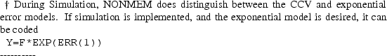
This is done because during data analysis NONMEM cannot
distinguish between the CCV error model
 and the exponential
error model
and the exponential
error model  , for which
 †. By using the
latter model and modelling the error in
†. By using the
latter model and modelling the error in
 rather than in
 , NM-TRAN enables PREDPP to
achieve an improvement in run time.
, NM-TRAN enables PREDPP to
achieve an improvement in run time.
----------
This is the error model (3.6):
Y=F+F*ERR(1)+ERR(2)
This is the error model (3.7):
Y=F+F**P*ERR(1)
The variable P must be assigned a value before its use
above. P is typically identified with an element of
 so that it can be estimated
in the fitting process. Let us assume that
so that it can be estimated
in the fitting process. Let us assume that
 is chosen for this purpose.
Then an alternative coding is:
is chosen for this purpose.
Then an alternative coding is:
Y=F+F**THETA(4)*ERR(1)
We have already seen how an indicator variable,
e.g., ASY, can be used in $PK statements for a variety of
purposes. The same technique is used in $ERROR statements.
Consider model 3.8 where the variable ASY has the value 1 or
0, corresponding to assay 1 or assay 2. ASY is a data record
item. Then the error model (3.8) is coded:
Y=F+ASY*ERR(1)+(1-ASY)*ERR(2)
In Chapter 3, Section 3.6, an example is given in
which there are two kinds of observations, plasma (
 ) and urine (
 ). With PREDPP,
measurements from different compartments of the model are
recorded in the DV data item of different observation event
records. The CMT data item identifies the compartment from
which the prediction associated with the event record is to
be obtained. When the $ERROR statements are evaluated for a
given event record, the variable F contains the prediction
from the compartment specified for that event record. All
that need be done is to select the correct error model,
depending on the compartment. Suppose, for example, that
ADVAN2 is used, so that the central compartment is
compartment 2 and the output (urine) compartment is
compartment 3. Then the error model (3.10) can be
coded:
). With PREDPP,
measurements from different compartments of the model are
recorded in the DV data item of different observation event
records. The CMT data item identifies the compartment from
which the prediction associated with the event record is to
be obtained. When the $ERROR statements are evaluated for a
given event record, the variable F contains the prediction
from the compartment specified for that event record. All
that need be done is to select the correct error model,
depending on the compartment. Suppose, for example, that
ADVAN2 is used, so that the central compartment is
compartment 2 and the output (urine) compartment is
compartment 3. Then the error model (3.10) can be
coded:
TYP=0
IF (CMT.EQ.2) TYP=1
Y=F+TYP*ERR(1)+(1-TYP)*ERR(2)
In Chapter 3, Section 3.7, an example is given in
which there are three kinds of observations. Suppose that
there are two data items, ASY1 and ASY2. ASY1 is 1 if assay
1 is used and 0 otherwise. ASY2 is 1 if assay 2 is used and
0 otherwise. This is the error model (3.11):
Y=F+ASY1*ERR(1)+ASY2*ERR(2)+(1-ASY1)*(1-ASY2)*ERR(3)