 : The $THETA Record : The $THETA Record


 and
and  : the $OMEGA and $SIGMA Records
 or
or 
 and
and 
NONMEM Users Guide Part V - Introductory Guide - Chapter 9
Chapter 9 - Additional NM-TRAN Records
This chapter tells how to give initial estimates to NONMEM’s parameters ($THETA, $OMEGA, $SIGMA records); how to tell NONMEM what tasks to perform ($ESTIMATION, $COVARIANCE records); and how to tell NONMEM what additional output to produce ($TABLE, $SCATTERPLOT records).
: The $THETA RecordThis record provides an initial estimate (and,
optionally, provides lower and upper bounds) for every
element of NONMEM’s  vector.
The $THETA record contains a list of values,
separated by spaces or commas, which are the initial
estimates for the  ’s
used in the $PK and $ERROR statements. The position of a
value in the list corresponds to its position (subscript) in
the
’s
used in the $PK and $ERROR statements. The position of a
value in the list corresponds to its position (subscript) in
the  vector. For example,
consider the following statement:
vector. For example,
consider the following statement:
$THETA 1.7 .102 29.
This says that the initial estimate for
 is 1.7, the initial estimate
for
is 1.7, the initial estimate
for  is .102, and the initial
estimate for
is .102, and the initial
estimate for  is 29. Some
users of NONMEM prefer to code each value on a separate line
so that they can include comments to themselves describing
the significance of the
is 29. Some
users of NONMEM prefer to code each value on a separate line
so that they can include comments to themselves describing
the significance of the  ’s. The above record could have been coded as
follows:
’s. The above record could have been coded as
follows:
$THETA 1.7 ; RATE CONSTANT OF ABSORPTION
.102 ; RATE CONSTANT OF ELIMINATION
19. ; VOLUME OF DISTRIBUTION
This is a matter of style.
When NONMEM is told to estimate the parameters
(Section 4.1, the Estimation Step, below), it varies the
elements of  to find values
which cause the model to fit the observations best. The
values on the $THETA record are the initial estimates of
to find values
which cause the model to fit the observations best. The
values on the $THETA record are the initial estimates of
 for this search. When only
an initial estimate is provided, NONMEM is free to chose any
positive or negative value for that element of
for this search. When only
an initial estimate is provided, NONMEM is free to chose any
positive or negative value for that element of
 . We then say that the
 element is
unconstrained, which means that its lower bound
(lower limit) is
element is
unconstrained, which means that its lower bound
(lower limit) is  and its
upper bound (upper limit) is
and its
upper bound (upper limit) is
 . When finite bounds are
desired, the initial estimate and its bounds must be
enclosed in parentheses and specified in the order (lower,
initial, upper). When the upper bound needn’t be
finite, the initial estimate and its lower bound are
enclosed in parentheses and specified in the order (lower,
initial). Note that when no estimation is performed, upper
and lower bounds have no effect.
. When finite bounds are
desired, the initial estimate and its bounds must be
enclosed in parentheses and specified in the order (lower,
initial, upper). When the upper bound needn’t be
finite, the initial estimate and its lower bound are
enclosed in parentheses and specified in the order (lower,
initial). Note that when no estimation is performed, upper
and lower bounds have no effect.
In the theophylline example of Chapter 2, for
example, negative  values
are physiologically impossible. Each
values
are physiologically impossible. Each
 element was given a lower
bound of 0, which constrained it to be
non-negative:
element was given a lower
bound of 0, which constrained it to be
non-negative:
$THETA (0, 1.7) (0, .102) (0, 29.)
It is possible to mix constrained and
unconstrained  s; this was
done in Chapter 2, figure 2.12:
s; this was
done in Chapter 2, figure 2.12:
$THETA (0,.0027) (0,.70) .0018 .5
An upper bound of
 may be stated explicitly
using the value 1000000 or the word
INFINITY. Similarly, a lower bound of
may be stated explicitly
using the value 1000000 or the word
INFINITY. Similarly, a lower bound of
 may be stated explicitly as
-1000000 or -INFINITY.
may be stated explicitly as
-1000000 or -INFINITY.
When estimation is performed, it is sometimes
desirable to hold one or more elements of
 to a constant value. One
example is when a full model is reduced to a simpler model,
as discussed in Chapter 5, Section 2.1; usually this is done
by holding some
to a constant value. One
example is when a full model is reduced to a simpler model,
as discussed in Chapter 5, Section 2.1; usually this is done
by holding some  element to
0. In fact, the value 0 may not be used as an initial
estimate for an element of
element to
0. In fact, the value 0 may not be used as an initial
estimate for an element of  unless this element is fixed to this value. A
 element is held constant by
inserting the word FIXED after the initial estimate.
For example, the following statement allows
element is held constant by
inserting the word FIXED after the initial estimate.
For example, the following statement allows
 and
and
 to vary, but holds
 to the value
.102:
to the value
.102:
$THETA 1.7 .102 FIXED 29.
Parentheses may be used to make the statement easier to
read:
$THETA 1.7 (.102 FIXED) 29.
If the lower, initial, and upper values for an element of
 are identical, the element
of
are identical, the element
of  is understood to be
fixed, even if the word FIXED does not appear.
is understood to be
fixed, even if the word FIXED does not appear.
When estimating parameters, good initial
estimates for  are sometimes
important. Poor initial estimates may occasionally cause the
NONMEM run to take excessive amounts of computer time, to
produce parameter estimates that are not physiologically
reasonable, or to fail to produce any parameter estimates at
all. For some drugs and models, initial estimates for
are sometimes
important. Poor initial estimates may occasionally cause the
NONMEM run to take excessive amounts of computer time, to
produce parameter estimates that are not physiologically
reasonable, or to fail to produce any parameter estimates at
all. For some drugs and models, initial estimates for
 can be obtained from
published literature describing prior studies with the drug.
For some studies, very accurate values may have been
obtained by prior runs with NONMEM or other regression
programs. Highly accurate values should be perturbed
(modified) by about 10% before being used as initial
estimates in a NONMEM run. (Initial estimates that are too
close to what may be the actual final estimates will cause
problems in a NONMEM run; see Chapter 13, Section 2.)
Sometimes, however, there is little guidance in choosing
initial estimates for some elements of
can be obtained from
published literature describing prior studies with the drug.
For some studies, very accurate values may have been
obtained by prior runs with NONMEM or other regression
programs. Highly accurate values should be perturbed
(modified) by about 10% before being used as initial
estimates in a NONMEM run. (Initial estimates that are too
close to what may be the actual final estimates will cause
problems in a NONMEM run; see Chapter 13, Section 2.)
Sometimes, however, there is little guidance in choosing
initial estimates for some elements of
 .
.
One approach with population data, where there is
a reasonable amount of data for each individual, is as
follows. It is often easier to guess at appropriate
parameter values for individual data than for population
data. So, first estimate each individual’s parameter
values using only the data from the individual. The mean
values of the individuals’ parameter estimates can
then be used as the initial parameter estimates in the
population analysis. Results from individual runs can also
be used to obtain initial estimates for elements of
 and
and
 ; see below.
Another approach is simply to let NONMEM find an initial estimate. NONMEM has an automatic strategy for so doing; see Chapter 12, Section 4.4.
and : the $OMEGA and $SIGMA RecordsRecall that  and
and
 are variance/covariance
matrices for the following random variables:
are variance/covariance
matrices for the following random variables:
Individual Model
|
|
Population Model
|
|
In all the examples in this document,
 and
and
 are diagonal
matrices, in which covariance elements such as
are diagonal
matrices, in which covariance elements such as
 (which is
 ) are assumed to be zero.
NONMEM also allows full variance/covariance matrices; this
is beyond the scope of this text, but see Chapter 12,
Section 4.1.
) are assumed to be zero.
NONMEM also allows full variance/covariance matrices; this
is beyond the scope of this text, but see Chapter 12,
Section 4.1.
Initial estimates for the variances must be
provided to NONMEM via the $OMEGA and $SIGMA records.
Initial estimates of all model parameters (
 ,
,
 , and
, and
 ) must be provided even if
estimation is not requested. $OMEGA and $SIGMA records each
contain a list of values, separated by spaces or commas,
which are the estimates for the corresponding variances. As
in the $THETA record, the position of a value in the list
corresponds to the position (subscript) of the corresponding
variance (along the diagonal) in the matrix.
) must be provided even if
estimation is not requested. $OMEGA and $SIGMA records each
contain a list of values, separated by spaces or commas,
which are the estimates for the corresponding variances. As
in the $THETA record, the position of a value in the list
corresponds to the position (subscript) of the corresponding
variance (along the diagonal) in the matrix.
With individual data,
 variables are used in
$ERROR records, where they are called either ERR or ETA. For
example, in the theophylline problem of Chapter 2 (figure
2.1) there appear the records:
variables are used in
$ERROR records, where they are called either ERR or ETA. For
example, in the theophylline problem of Chapter 2 (figure
2.1) there appear the records:
$ERROR
Y=F+ERR(1)
$OMEGA 1.2
Here, ERR(1) corresponds to  , and the initial estimate for its variance is 1.2: i.e.,
 .
.
With population data,
 variables are used in $PK
statements. For example, in the phenobarbital problem of
Chapter 2 (figure 2.6) there appear the
lines:
variables are used in $PK
statements. For example, in the phenobarbital problem of
Chapter 2 (figure 2.6) there appear the
lines:
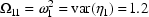
CL=TVCL+ETA(1)
V=TVVD+ETA(2)
$OMEGA .0000055, .04
The $OMEGA record says that the initial estimate for the
variance of  is
is
 , and of
 is .04: i.e.,
 and
and
 . Some users of NONMEM
prefer to code each value on a separate line so that they
can include comments:
. Some users of NONMEM
prefer to code each value on a separate line so that they
can include comments:
$OMEGA .0000005 ; VARIANCE IN CL
.04 ; VARIANCE IN V
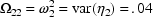
This record is used only with population data,
and is similar to the $OMEGA record. It gives the initial
estimates of the variances of the
 variables used in the
$ERROR statements, where they are called either ERR or EPS.
For example, in Figure 2.6, there also appears the
records:
variables used in the
$ERROR statements, where they are called either ERR or EPS.
For example, in Figure 2.6, there also appears the
records:
$ERROR
Y=F+ERR(1)
$SIGMA 25
Here, ERR(1) corresponds to  , and the initial estimate for its variance is 25: i.e.,
 .
.
or It is sometimes desirable to hold one or more
elements of  or
or
 to constant
value(s).
to constant
value(s).
In the population example of Chapter 2 it is
possible to ignore interindividual variability in CL by
fixing  to 0†.
----------
The variance of an
 or
or
 variable is held constant
by inserting the word FIXED after the initial
estimate:
variable is held constant
by inserting the word FIXED after the initial
estimate:
$OMEGA 0 FIXED .0225
Parentheses may be used to make the statement easier to
read:
$OMEGA (0 FIXED) .0225
As with  , the value 0 may
not be used as an initial estimate for any element of
, the value 0 may
not be used as an initial estimate for any element of
 or
or
 unless the element is fixed
to this value.
unless the element is fixed
to this value.
and The initial estimates for the variances will
depend on the particular (interindividual and/or
intraindividual) error models chosen. The estimates do not
have to be particularly accurate, although values which are
much too small can cause difficulties for NONMEM. In
general, it is better to over-estimate the variances rather
than to under-estimate them. As with initial estimates for
 , initial estimates can
sometimes be obtained from published literature or from
prior runs with NONMEM or other regression
programs.
, initial estimates can
sometimes be obtained from published literature or from
prior runs with NONMEM or other regression
programs.
Initial estimates can also be obtained by an
approach which we illustrate with examples for both
intraindividual and interindividual error models. The
standard deviation of a physiological quantity is generally
some fraction  of its
typical value
of its
typical value  :
:
 .
.
For the additive model:


Some ambiguity exists about what we mean by
"the typical value" of y. For the purpose of
obtaining an initial estimate of the variance, we need not
be too particular about this. For the theophylline example
(Figure 2.1), we may choose the mean of the observed values
as the typical value. This value is approximately 5.4.
Assuming 20% error, i.e.  ,
then
,
then  . Similarly, in the
first phenobarbital example (Figure 2.6), the mean of the
observations is approximately 25. Again assuming 20% error,
then
. Similarly, in the
first phenobarbital example (Figure 2.6), the mean of the
observations is approximately 25. Again assuming 20% error,
then  , and
, and
 . For that same example,
the typical value of CL was estimated according to the model
for the parameter: TVCL=THETA(1). We used the
initial estimate of
. For that same example,
the typical value of CL was estimated according to the model
for the parameter: TVCL=THETA(1). We used the
initial estimate of  ,
.0047, as the typical value of CL, and assumed 50% error:
,
.0047, as the typical value of CL, and assumed 50% error:
 . The model for V is
TVVD=THETA(2). Again, we used the initial estimate
of
. The model for V is
TVVD=THETA(2). Again, we used the initial estimate
of  , .99, as the typical
value of V, but assumed 20% error:
, .99, as the typical
value of V, but assumed 20% error:
 . Note finally that in the
second phenobarbital example (Figure 2.12), we used as
initial estimates of variance the final estimates obtained
from the first example (understanding that these estimates
could be somewhat large due to some of the variability being
explained in this example by a systematic influence of
weight).
. Note finally that in the
second phenobarbital example (Figure 2.12), we used as
initial estimates of variance the final estimates obtained
from the first example (understanding that these estimates
could be somewhat large due to some of the variability being
explained in this example by a systematic influence of
weight).
For the constant coefficient of variation model:


If we identify t with the value of f (whatever it may be), we have:

In other words, using the CCV model, we do not
need to estimate the typical value of the variable. For
example, assuming 20% error,
 .
.
As with  , it is
possible for NONMEM itself to obtain initial estimates of
, it is
possible for NONMEM itself to obtain initial estimates of
 and
and
 automatically; see Chapter
12, Section 4.4.
automatically; see Chapter
12, Section 4.4.
Two main tasks of NONMEM, the Estimation Step and the Covariance Step, are optional and must be specifically requested by including the $ESTIMATION and $COVARIANCE records. To skip the Estimation Step, simply omit the $ESTIMATION record. To skip the Covariance Step, simply omit the $COVARIANCE record.
In every run NONMEM computes and prints the value of the objective function and the final parameter estimates. The values printed are based on the final parameter estimates if the Estimation Step is requested, and are based on the initial estimates if it is not.
In the Estimation Step, NONMEM performs a search
to obtain those values of  ,
,  , and (for population
studies)
, and (for population
studies)  which give the
lowest value of the objective function. The output of this
step is the pages whose titles are " MONITORING
OF SEARCH: ", " MINIMUM VALUE OF
OBJECTIVE FUNCTION ", and " FINAL
PARAMETER ESTIMATE ". This step is requested by
the presence of the following statement:
which give the
lowest value of the objective function. The output of this
step is the pages whose titles are " MONITORING
OF SEARCH: ", " MINIMUM VALUE OF
OBJECTIVE FUNCTION ", and " FINAL
PARAMETER ESTIMATE ". This step is requested by
the presence of the following statement:
$ESTIMATION
There are several options, which are described in the NONMEM
Users Guide, Part IV. The most frequently used ones are as
follows.
SIGDIGITS=n
|
By default, the search continues until the
estimates of all elements of
|
MAXEVAL=n
|
The Estimation Step always runs with a specific limit on the number of objective function evaluations allowed during the search, as a protection against infinite loops and excessively long runs. The default maximum is computed according to the number of parameters being estimated. The MAXEVALS option can be used to request a different number (n) for the maximum number of function evaluations. |
PRINT=n
|
As the Estimation Step progresses, by default it
prints intermediate output summarizing the progress of the
search. The search proceeds in stages, called iterations. At
the end of certain iterations a summarization is printed
which consists of the values of the objective function, its
gradient vector with respect to the parameters, and the
parameter values themselves. By default, this summarization
is only printed for the first and last iterations. The PRINT
option can be used to request a number (n) such that
starting from the first iteration, only n-1 iterations are
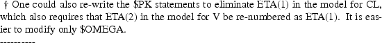
skipped before another summarization is printed†. |
An example of the use of these options
is:
$EST SIG=6,MAX=900,PRI=5
In addition to the first and last iterations, summarizations
are printed every 5th iteration. Notice that abbreviations
of the record and option names were used; this is a matter
of style.
In the Covariance Step, NONMEM obtains
information on the precision of the parameter estimates
obtained in the Estimation Step. The output of this step are
pages with titles " STANDARD ERROR OF
ESTIMATE ", " COVARIANCE MATRIX OF
ESTIMATE ", " CORRELATION MATRIX OF
ESTIMATE ", and " INVERSE
COVARIANCE MATRIX OF ESTIMATE ". This step is
requested by the presence of the following
record:
$COVARIANCE
There are several options, which are discussed in NONMEM
Users Guide, Part IV. The Covariance Step cannot be
requested by itself; the Estimation Step must precede
it‡.
----------

$TABLE and $SCATTERPLOT records are used to request NONMEM steps which generate additional output. If one of these records is omitted, NONMEM does not produce the corresponding additional output. Tables and scatterplots are generated after all other tasks have been performed. This affects the values displayed for PRED, RES, and WRES. If the Estimation Step is not run, then the initial estimates of the parameters are used to compute these quantities. If the Estimation Step is run, then the final parameter estimates are used. Residuals (RES) and weighted residuals (WRES) are defined in Chapter 11, Section 4.4.2.
The UNCONDITIONAL option of the $TABLE and $SCATTERPLOT records requests that output of this type be generated even if the Estimation Step terminates unsuccessfully, and is the default. The CONDITIONAL option of these records requests that output of this type be generated only if the Estimation Step terminates successfully.
The values of DV, PRED, RES, and WRES are always
printed in every table. Other data items to be printed
should be listed on the record. The data items are printed
in the order in which they are listed. This does not have to
be the same order as in the data file, nor does every data
item have to be listed. For example, the following record
appears in Chapter 2, figure 2.12:
$TABLE ID TIME AMT WT APGR
Figure 10.10 in Chapter 10 shows a portion of the resulting
output.
It is possible for the lines of a table to be sorted into a different order than that of the original input file; this is discussed in the NONMEM Users Guide, Part IV.
More than one table can be printed. A separate $TABLE record is used to request each one.
Chapter 2 contained many examples of $SCATTERPLOT
records and the resulting output. Here, for example, are the
records from figure 2.6:
$SCATTERPLOT PRED VS DV UNIT
$SCATTERPLOT RES VS WT
The word UNIT requests a unit-slope line, which is the line
PRED=DV. Figures 2.10 and 2.11 show the resulting
output.
Similarly, the word ORD0 can be used to request a zero line on the ordinate axis.
It is possible to generate several scatterplots
with a single record, by using a list of data item
names:
$SCATTERPLOT (PRED,RES,WRES) VS WT
This produces three scatterplots, and has the same effect as
the three records:
$SCATTERPLOT PRED VS WT
$SCATTERPLOT RES VS WT
$SCATTERPLOT WRES VS WT
Sometimes it is desirable to partition a
scatterplot into a number of separate scatterplots. For
example, if the data contain both plasma and urine
observations, it would be better to separate the scatterplot
of PRED vs. DV into one scatterplot where the DV values are
the plasma observations, and another one where the DV values
are the urine observations. To do this, it is necessary to
specify a partitioning data item, in this case, the CMT data
item, which gives the compartment number of the observation.
The following record could be used.
$SCATTERPLOT PRED VS DV BY CMT UNIT
This will produce separate scatterplots: one with plasma
observations (CMT=1 if ADVAN1 is used), and one with urine
observations (CMT=2 if ADVAN1 is used).
Two partitioning items can also be
specified:
$SCATTERPLOT PRED VS DV BY CMT SEX UNIT
One scatterplot is produced for each unique
combination of values of the two partitioning data
items.
Two main rules control the placement and order of records within a NM-TRAN control file:
|
The $INPUT record must appear before any records which contain data item names ($PK, $ERROR, $TABLE, $SCATTERPLOT) The $SUBROUTINE, $PK, and $ERROR records should appear in the indicated order, but do not have to be consecutive. |
The records $DATA, $THETA, $OMEGA, $SIGMA, $ESTIMATION, $COVARIANCE, $TABLE, and $SCATTERPLOT can be placed anywhere among the control records, in any order. However, NONMEM always performs its tasks in a fixed order:
|
Estimation Step |
Thus, even if the $TABLE record precedes the $ESTIMATION record, the values of PRED, RES, and WRES in the table will be based on the final parameter estimates.
 (OMEGA) for
 (Random Intraindividual
Variability)
(Random Intraindividual
Variability) (OMEGA) for
 (Random Interindividual
Variability)
(Random Interindividual
Variability) (SIGMA) for
 (Random Intraindividual
Variability)
(Random Intraindividual
Variability) ,
,
 , and
, and
 have been determined to at
least 3 significant figures. Because only 3 significant
digits are used to print parameter estimates in the output,
and for other reasons as well, this amount of accuracy is
often sufficient. However, the SIGDIGITS option can be used
to request a different number (n) of significant
digits.
have been determined to at
least 3 significant figures. Because only 3 significant
digits are used to print parameter estimates in the output,
and for other reasons as well, this amount of accuracy is
often sufficient. However, the SIGDIGITS option can be used
to request a different number (n) of significant
digits.